Financial Markets

Last time we did the goods market. Now it’s the financial market’s turn. This one’s also “short-term” — as in, it’s a short-term model.

OK so. The variables we hadn’t touched yet — money and the interest rate… We’re going to look at the financial market through these.

The thing is, a variable like money supply clearly isn’t something that runs the goods market — at least not in the model we just built — but it’s a huge deal for the financial market. That’s why we split the financial market off from the goods market and look at it separately.

(Yeah yeah, my wording’s a bit clunky….. but as we go, you’ll see why splitting goods and financial markets makes sense. And eventually, we mash the two back together to build a single AD — aggregate demand. Don’t worry, don’t worry.)

OK, OK. Say you’ve got 50,000 won saved up. There’s nowhere particular you need to spend it. (Remember earlier — we said all this money ends up as savings.)

What’s the smart thing to do with it?

At this point, your options are basically:

1. Just hold it as cash?
2. Dump it in a bank deposit?
3. Buy bonds?
4. Buy stocks?

(The sky-blue ones are what people usually call “money.”)

So basically — we’re going to agonize over “how should I hold it?” Meaning: what form do I keep my money in?

From here on, our whole perspective sits on this thing called “money.” And the question we ask is:

“How much do people want to hold as money?” → “Demand for money”

This money demand depends on two variables: “transaction volume” and the “(bond) interest rate.”

And “transaction volume” — the amount you transact… Look, it’s not weird at all to say: if my nominal income jumps 10%, the amount I transact jumps 10% too. (We can say this confidently.) So let’s just go ahead and assume transaction volume is proportional to nominal income!

In words — money demand is proportional to nominal income. Now I want to upgrade this into an actual Equation. (Which means we need a proportionality constant.)

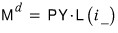
Let’s (also) assume that what links these two — the proportionality constant — is determined by an “interest rate function.” You at least need to find this assumption somewhat believable — and it’s not crazy. It would be absolutely insane to drag along a formula you yourself don’t even buy!?

(The reason we can write PY = nominal income → again, ∵ the ’three-sided equivalence principle of national income’ (equilibrium total production = equilibrium total expenditure = equilibrium total income).)

A small thing to add —

these two statements actually say different things. The first one says nominal income and money demand have a (+) relationship — but not necessarily proportional. The second one says yeah, the (+) relationship is there, AND, more strongly, it’s proportional.

But like I said up top, since we can say transaction volume and nominal income are proportional, we go with the stronger second version. (Honestly, it just makes more sense, right?)

Why L? Because L is from Liquidity. So — it’s a liquidity function. What “liquidity” actually means, I’ll keep going on later.

And the meaning of that little (-) subscript, simply put: if the interest rate drops, people want to hold more money. Meaning the value of the liquidity function goes up. If the interest rate rises, people want to hold less money, meaning the liquidity function value goes down. It’s saying: negative relationship… negative relationship.

OK so,

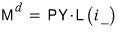
we can also read this equation as: (with nominal income held constant) the variable that determines “money demand” is the interest rate i!

OK, then by the same logic as last post, “Equilibrium — whatever it is, at any given moment, supply and demand have to match~”

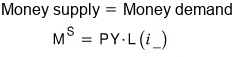
Let me twist the interpretation a little. What this equation is saying is:

When nominal income is constant, the interest rate i is what gets determined to balance against the existing money supply.

(I keep saying “nominal income is constant” — and to hammer this home one more time: this is a short-term model, so this assumption isn’t some wildly bizarre one!)

So this equilibrium relation between L (liquidity) and M (money supply) — we call it the LM relationship. And then, depending on how the monetary authority cranks the money supply up or down, we can say “ah, the interest rate gets determined like this, like that,” and one of the methods for how the monetary authority moves the money supply is open market operations (OMO). For the full story, honestly just check out ‘My Studies in Monetary Finance’ — it’s got way, way more than enough.

cf. Policy of increasing the money supply: expansionary policy. Policy of decreasing the money supply: contractionary policy.

One more aside for reference. When the central bank actually runs monetary policy, what it almost always uses is Repo…. (go go My Studies in Monetary Finance) That’s the simple textbook picture; central banks today also steer short rates directly through the rates they pay and charge, so read this as the model’s version.

Anyway — they use repo bonds to crank money supply up or down, so the “interest rate” we keep talking about is the interest rate on bonds. But the interest rate on bonds isn’t actually a number that’s set in stone somewhere — it’s something derived from the price of bonds, and that derived value is what we recognize as the interest rate.

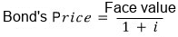
That’s how the interest rate is set — at least in the simplest case, a one-year bond that pays only its face value at the end.

(I’m being super sloppy here — go go My Studies in Monetary Finance.)

I’m bringing this up because I want to explain why an open market purchase (= releasing money) causes the interest rate to drop.

The mechanism: open market purchase → bonds↓ & money↑ (in the public’s hands) → bond demand↑ → bond price↑ → interest rate↓

So — bond price and the interest rate are inversely related!

OK, so when you occasionally see in the news, “We’re setting the benchmark interest rate at x%~” — that doesn’t mean the central bank governor utters the words and poof, the rate is what it is. It means the moment that order goes out, a hundred or so central bank employees are out there buying and selling RP — ahh, repo.

That is, the central bank stares at the demand curve and goes “Oh ho, if we release about this~ much money supply, the equilibrium rate will land here, so let’s set our supply quantity to !” — apparently that’s how it goes down.

And the interest rate set this way isn’t just any interest rate — it’s a short!-term! interest rate. Let’s leave it at that for here, and please go to My Studies in Monetary Finance for more.

Now we’ll extend this LM relationship model one step further to derive the LM curve. The plan: start from the public’s demand for money (cash and deposits) and work out from it the demand for the money the central bank issues.

So what do I mean by “extending the model”?

The fact is — money can exist in two forms. That’s the direction I want to expand in. Earlier we treated money as cash only, but now we’ll also bring “demand deposits” into the picture.

So total money demand is 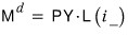same as before. But we’ll split it: the amount people want to hold as cash & the amount people want to hold as demand deposits. <Because cash is better for small payments, deposits are better for large ones.>

So let c be the share of total money people want to hold as cash, and then automatically the share they want to hold as deposits is 1-c (since we’re saying these are the only two forms.) Now let’s build this into an equation.

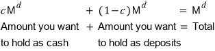
The “amount people want to hold as deposits” we just got, , ties directly into the bank’s “demand for reserves.” When an amount equal to this rolls in as deposits, the bank has to make a call. “Hmmm ~ ~ out of this much money, how much do I stack in the vault and how much do I lend out?!”

Because of unpredictable deposit and withdrawal flows & the legal reserve ratio (10% in the US, 7% in South Korea, when this was written), each bank apparently stacks up reserves at a higher rate than the legal minimum, in their own way. We’ll call that bank’s individual reserve ratio θ.

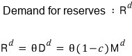
OK, that’s the whole story. “Total money” demand is

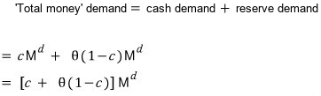
Now — about “total money”: what the central bank issues, as you’d know from My Studies in Monetary Finance, isn’t just plain “money” — it’s called the monetary base, also known as high-powered money. So is the thing.

The (US-standard) Federal funds rate is the interest rate that gets determined against this and this , and it’s called the interbank (ultra-)short-term interest rate.

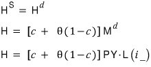
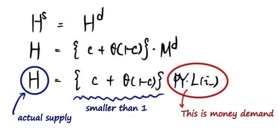
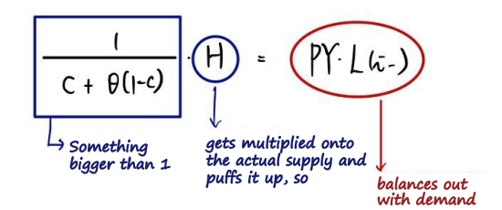
OK then — if the central bank’s money supply is , equilibrium with demand looks like:

I was going to derive the IS curve and the LM curve right here, but the post has ballooned again for no good reason… sorry about that. Derivation of the IS curve and LM curve — I’ll pick that up in the very next post.