Wage Setting and Price Setting

In the previous post,

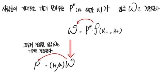
we got up to here.

I felt like if I just kept barreling all the way to the end, the thing would get waaaay too long and saggy, so I deliberately cut it off.

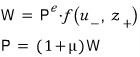
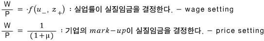
Let me rewrite it cleanly with the equation tool.

OK, now picking up right where we left off.

So I’m gonna make an assumption.

What assumption, you ask —

This one.

Actually, calling it an “assumption” is a bit of a stretch.

In the medium run, at equilibrium, the expected price level and the actual price level end up coinciding.

I’ll get to why below.

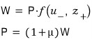
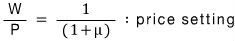
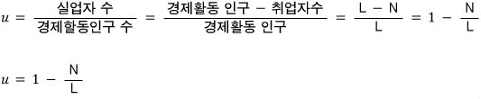
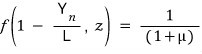
And I’ll massage the expression into this:

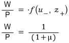
W/P — from now on let’s read this as the “real wage.”

Then we can say the following:

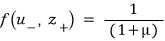
And now I’m gonna draw this thing as a graph,

zooming in on the variables we actually care about — real wage and unemployment rate — and putting them on the x and y axes.

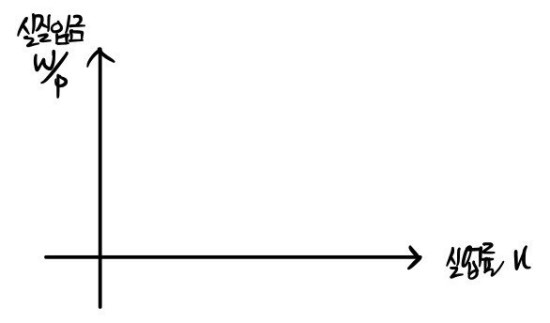
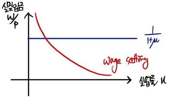
Here are the axes. (x-axis is unemployment rate u, y-axis is real wage W/P.)

First, drawing in the wage setting:

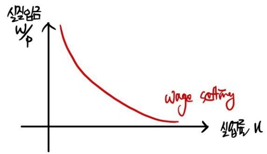
It looks like this.

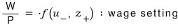
The function f() — its values get smaller as u gets bigger, right?

So now you’ve gotta sit with this:

Why isn’t it a straight line, why a curve? And among curves, why convex downward and not convex upward?

Honestly? I can’t answer that right now. To say anything about slope you’d need to differentiate,

and… we don’t actually have an expression to differentiate, do we????

So all we can really do is read it like this:

“The bigger u is, the smaller the rate of decrease of real wage per unit increase in unemployment rate.”

…heh. Does that make sense? Anyway, moving on.

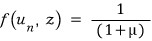
Now we need to draw this in.

Easy, right? This function doesn’t depend on u at all.

High unemployment, low unemployment — doesn’t matter. The real wage gets determined purely by the markup.

I’ll draw it into the graph above like this:

Oh — an intersection?

What’s the expression at the intersection?

Obviously this!

Because the values match exactly!!!!

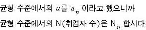
The unemployment rate u at this intersection —

— we grab the n from “nature” and write it this way,

and let’s read it as “natural unemployment rate”!!!!

• Why we write it like that and read it like that? Will become clear in a sec.

For now, we can say this much:

Meaning: once a firm sets its μ (mark-up), the unemployment rate u that pops out as a result — that’s what this is referring to.

OK so we’ve got the graph drawn.

The factors that shift wage setting — changes in z,

and the factors that shift price setting — changes in μ —

we can now check out how the natural unemployment rate

(the equilibrium point) shifts around accordingly~

Quick sketch:

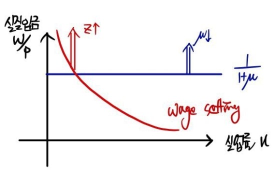
When z goes up, wage setting shifts upward.

And when μ goes down, that’s when we say price setting shifts upward~~~

Now, one thing we absolutely cannot forget is that

that intersection sitting there

is the intersection under the condition that this holds!!!! Don’t lose track of that.

OK then. Now I wanna convert our variable u (unemployment rate) back into “employment.”

Why am I bothering? I’m not telling you!!!! >_<

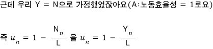
Let’s rewrite it like this.

With that rewrite, if we write the equation at the equilibrium point again,

this thing

let’s write as this.

And lemme say a little something about what this expression actually means.

is the natural unemployment rate determined by the circumstances of society.

The output at that point is what we call

“potential output.”

If our society’s efficiency were so extraordinary that the unemployment rate landed exactly at

then the output

is what we’d be sitting at —

but our society isn’t that efficient,

so

is, realistically, a dream-level output.

Cranking society’s “efficiency” up to the max and pushing output toward

— that’s society’s goal.

And finally, just to hammer it home one more time —

in conclusion:

at the intersection of the price-setting curve and the wage-setting curve, the Y value is

and at that point the price level is

Once more:

when

the price level is exactly~~~!!!!!!!

that.

OK, we’re almost at the destination.

The real destination, actually, is to build the AD curve and the AS curve~~~~?!

Aggregate Demand, Aggregate Supply —

i.e., constructing the aggregate demand curve and the aggregate supply curve.

Buuut if I keep going from here this post is gonna get really long again.

Gonna stop here and pick it up fresh in the next post~!!

Originally written in Korean on my Naver blog (2016-01). Translated to English for gdpark.blog.