Okun's Law

Alright, the moment has finally arrived.

Remember how our AD-AS model couldn’t explain inflation? Yeah. Time to fix that!!!

Up to this point we’ve been thinking about the whole economy with just price level $P$ and output $Y$ — squeezing AD and AS into that two-variable picture. Now we’re going to slide a new variable into the mix: inflation, $\pi$.

Step one on that journey: Okun’s law.

In one sentence: Okun’s law is not the relationship between $\pi$ and $Y$. (Sorry.) It’s the relationship between the unemployment rate $u$ and economic growth $\Delta Y$. We’ll get to inflation in a sec — Okun is the bridge.

Anyway, let’s dig in.

Last chapter we assumed labor productivity was $A = 1$ and rolled with $Y = NA$.

(Here $L$ is the economically active population, $N$ is the number of employed people.)

OK OK OK OK, so with $A = 1$ we just have $Y = N$. Which means: if $Y$ changes by, say, $x\%$, then $N$ — the number of employed people — also changes by exactly $x\%$.

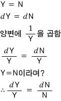
If $Y$ changes by $x\%$, $N$ changes by $x\%$.

So far so good, right?

Cool — let me start pulling formulas out one by one.

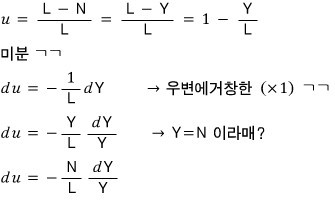
In plain words, here’s what this is saying:

The change in the unemployment rate is (negatively) proportional to the change in output relative to output — which is just the economic growth rate, right?

So: economic growth and unemployment move in opposite directions, proportionally.

(Quick aside. $N/L$ is technically the employment rate. So if you read it straight off the equation, the proportionality constant between economic growth and unemployment came out to be the employment rate. But in the real world the employment rate is NOT actually a proportionality constant in this relationship.

Why not? Probably because our assumptions baked the world into something way too clean and simple…

So I’d say: don’t read $N/L$ as “the employment rate” here. Read it as just “some proportionality constant” and move on.)

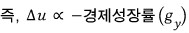
Why $g(y)$ with $g$ and $y$ as subscripts? Just think growth rate of yield and that’s your mnemonic.

Now let me rewrite that proportional relationship while bolting on a time dimension.

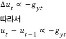
$g(y_t)$ is the rate of change of $Y$ in year $t$ relative to $Y$ in year $t-1$. Aka the economic growth rate of year $t$. heh heh heh.

Now apparently — that’s what the textbook says — the U.S. economy in the 1970s is well described by

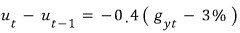
this exact formula.

Which is kind of cool, because it means the proportional relationship we just cooked up from those weirdly-clean assumptions is not as silly as it looked.

So!

Since this formula apparently nailed the society of that era, let’s stare at it for a sec and ask what it implies.

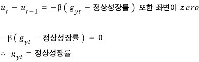
i) For $\Delta u = 0$ — meaning the unemployment rate stays the same as last year, i.e. doesn’t change at all:

The economic growth rate in year $t$ has to be 3%!!!

ii) If the economic growth rate is greater than 3%:

Unemployment in year $t$ is less than in year $t-1$. Unemployment falls.

iii) If the economic growth rate falls short of 3%:

Unemployment in year $t$ is greater than in year $t-1$. Unemployment rises.

That magic 3% — the economic growth rate that keeps unemployment exactly steady — has a name. It’s called the normal growth rate (or normal economic growth rate).

OK so we said Okun’s law is the relationship between unemployment and economic growth, right? Then this U.S.-1970s formula is exactly what’s expressing Okun’s law.

But the specific numbers — 0.4, 3% — those are obviously going to be different country to country, right?!

So let’s rewrite the formula in general form.

Boom. That’s Okun’s law in its general equation form.

Just to hammer it home one more time: Okun’s law is the relationship between $u$ and $g(y)$.

From here on it’s a mix of recap and new stuff!!! Could get a little dizzying so brace yourself.

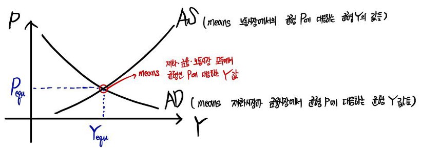
First — going back to the aggregate demand / aggregate supply model from earlier — there’s a relationship in there we never bothered to write out cleanly.

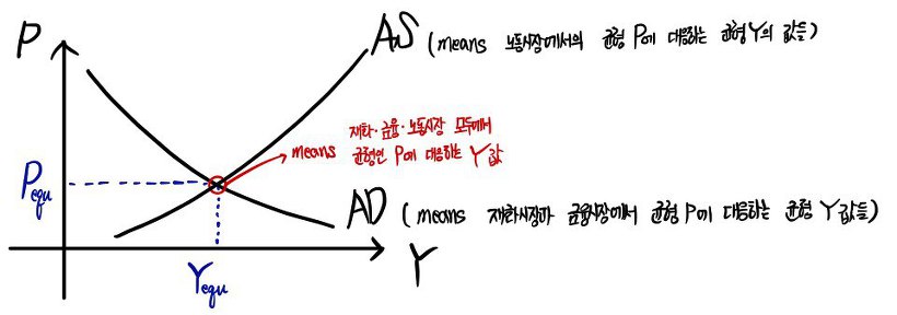
Namely: the relationship between inflation and the rate of change of $Y$ — i.e. inflation and economic growth.

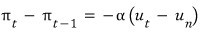
And the Phillips curve, which we just learned literally one chapter ago: that was the relationship between inflation and unemployment.

And and and — we can also pull the relationship between the rate of change of nominal money supply and economic growth straight out of the Aggregate Demand relationship. Let me actually show that one.

AD is

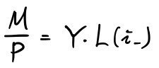
— that’s how we built it, right?

Let me write it loosely as

with $\gamma$ positive and (say) constant.

(When the interest rate is constant, $Y$ and $M/P$ are in a (+) proportional relationship right out of the gate, so I think we’re fine treating it this way.)

Now let’s mess around with that formula. I’m going to treat $M$ and $P$ as variables and use partial derivatives — two-variable function style — so don’t freak out.

(If you don’t know what partial differentiation is, hit me up. I’ll literally take a photo of the partial-differentiation section of my math textbook and send it to you. It’s not a brutal concept!!! There were even high school math teachers who taught it.)

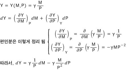
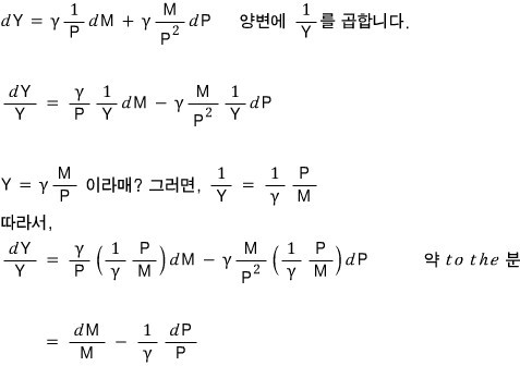
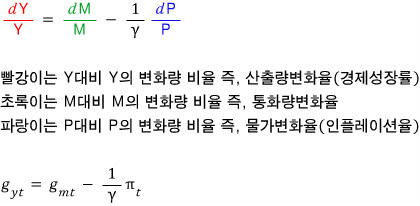
In $g(m_t)$, the $m$ is monetaryyy — rate of change of money supply in year $t$. We good?!

Summary

○ Relationship between inflation and economic growth: from the AD–AS relationship

○ Relationship between unemployment and inflation: the Phillips curve

○ Relationship between economic growth and unemployment: Okun’s law

○ Relationship between the rate of change of nominal money supply and economic growth:

OK, let me read these together and see what falls out.

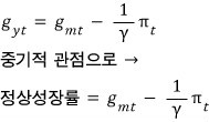
Medium-term view

Let’s look at it from a medium-term perspective.

Way back when we did the medium-term stuff, we said in the medium term

holds. Plug that into the Phillips curve first:

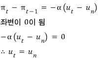
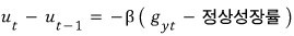
So in the medium term, the unemployment rate coincides with the natural rate of unemployment.

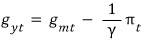
Now let me apply the same idea to Okun’s law.

That’s saying: this relationship holds in the medium term.

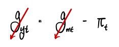
Now plug that into our unnamed-fourth-formula, the “rate of change of nominal money supply vs. economic growth”:

※ Just suppose ※

What if the monetary authority pins the rate of change of nominal money supply at

as a constant?!?!?!

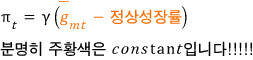
So in the medium term, if the rate of increase of nominal money supply is held constant,

rate of increase of nominal money supply $-$ normal growth rate $=$ inflation rate.

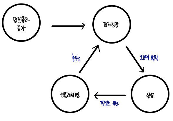
We’ve actually seen this kind of result before. Changes in (nominal) money supply have zero effect on output $Y$ or unemployment $u$ — they only show up in the price level $P$ / inflation $\pi$. Remember?

But — and this is the part you absolutely cannot mix up — that was from a “medium-term perspective.” The assumption that pinned us into the medium-term view was

this one.

So with results like this, Milton Friedman famously said:

“Inflation is always and everywhere a monetary phenomenon.”

Corporate monopolies, powerful labor unions, strikes, fiscal deficits, rising oil prices — name as many factors as you want. As long as they don’t move the rate of increase of nominal money supply, they have no effect whatsoever on inflation in the medium term. Apparently.

Short-term view

Now let’s swing over to the short term. For consistency of logic I’m going to lean on Chapter 7 stuff.

Say the monetary authority lowers nominal money supply.

By the IS-LM relationship, the AD curve shifts left.

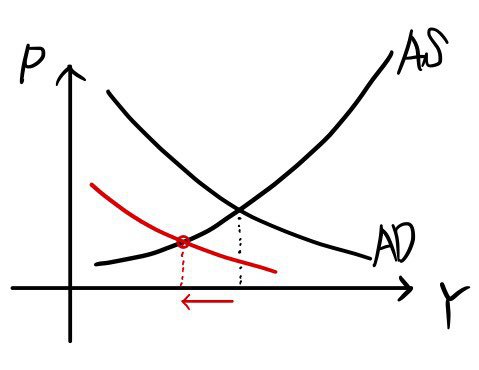
So $Y$ decreases.

This is exactly what falls out of our fourth formula — the “relationship between the rate of change of nominal money supply and economic growth.”

It was sitting inside this. (For now, hold inflation constant.)

Monetary authority lowers money supply $\Rightarrow$ economic growth rate falls. Then by Okun’s law,

$\Delta u$ goes up. Unemployment rises.

And because unemployment rose,

via the Phillips curve, inflation drops.

Viewed in this light — yeah, it makes total sense that the government (whose top priority is employment stability) and the central bank (whose top priority is price stability) are basically always at each other’s throats. If they weren’t fighting, that would be the genuinely weird society.

Cool. Now from that short-term state, let’s connect the dots back to the medium term.

First, the AS curve will shift and output will return to $Y_n$. So the economic growth rate $g(y_t)$ returns to the normal level, $\Delta u$ goes back to $0$, and $\Delta \pi$ also goes back to $0$.

But by this point the price level has dropped, so $|\pi|$ has gotten smaller, right?

So the textbook puts it this way:

“In the short term, monetary tightening causes a deceleration of growth and a temporary rise in unemployment.

In the medium term, the economic growth rate returns to normal and the unemployment rate returns to the natural rate of unemployment.

The monetary growth rate and the inflation rate are both permanently lower at this point.

Whether or not that’s the right way to put it — it’s as if one has bought a permanent decline in the inflation rate at the cost of a temporary rise in unemployment.”

Vocab note

• Deflation: a fall in the price level — i.e. a (negative) inflation rate.
• Disinflation: a fall in the inflation rate ($\pi$).

Don’t mix these two up.

Originally written in Korean on my Naver blog (2016-01). Translated to English for gdpark.blog.