The Relationship Between Savings Rate and Output

In the last post, we decided that “output per person” was going to be our indicator of economic growth.

(Translation: if output per person goes up, we call that economic growth.)

And once we started chasing that thing — output per person — we ended up concluding that it depends on capital per person ($K/N$) and the level of technology ($F(\sim)$).

So in the next chapter — chapter 11 — we go after $K/N$, and then over chapters 12 and 13 we apparently go after “technology.”

Alright. Into chapter 11 we go.

$K/N$, the amount of capital per person — we’ve been thinking of this as “the scale of capital.”

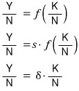
We said output per person $Y/N$ is

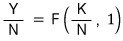
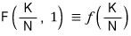
and just to keep the notation clean, we’re going to write

OK and to keep the thinking simple, let me toss in a couple of assumptions.

※ Heads up: Assumptions ※

“Population size and the labor force participation rate are constant.”

Under this assumption, we can treat $N$ as a constant. (I don’t actually picture $N$ as nailed-down-forever in the long run — I think of it more as a dynamic equilibrium where, at any given moment, the number of people retiring equals the number of people newly getting hired. I just made that English phrase up on the fly lol, no idea if that’s the proper way to put it.)

Under this setup, we don’t really need to keep emphasizing the “per person” part anymore.

I’ll just write or not-write the “per person” notation depending on my mood lol.

Second assumption:

※ Heads up: Assumptions ※

The function $f$ doesn’t depend on time.

Translation: just think of the level of technology as constant.

Trying to model this as a dynamic equilibrium too would get messy fast, so let’s just pretend the technology level isn’t doing anything dramatic.

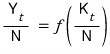
On top of these assumptions, let’s add a time dimension.

Rewriting the equation:

Alright. The thing we want to think about is $K$. $K$ is “capital.”

But capital isn’t only “money.”

An office is capital. Machinery, factories, the works — all capital.

So we want to roughly split capital $K$ into two flavors:

Flow & Stock

The difference between flow and stock is whether or not it depends on “time.” (cf. money is a stock, income is a flow. You’ve heard things like that, right?)

A few more examples:

• flow: output, savings, investment, etc.
• stock: employment, capital, etc.

OK so what we want to look at right now is “investment.”

The savings rate is going to differ country to country.

And it’s fair to say $K$ wobbles around according to that “savings,” right?!

To dig into the connection with savings, let’s drag back the assumptions we made waaay at the start (around chapter 3?) — closed economy ($NX = 0$) and $G - T = 0$ — and then

boom!!!!

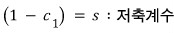
But private savings $S$ depends on each person’s income. (Remember? We did all of this already.)

Because of that, we call the proportionality coefficient the “savings coefficient,” and

is what we called $1 - \text{mpc}$…

So,

setting it like this,

$$I = sY$$

we can write that, and

and slapping the time axis on too,

— up to here, that was all flow.

From now on, we go after stock.

So $K$ is both a flow and a stock thing. The $K$ from year $t$ has been depreciated by $\delta$ —

subtract that off,

and that is what flows into $K$ for the following year,

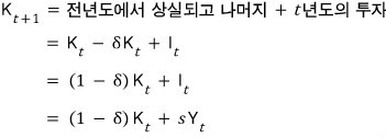
— so we can say. That is,

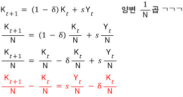
We’re going to play around with that equation up there.

Let me walk through the red equation we just got:

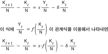
Now we’re going to express it like this. Don’t miss this.

You can rewrite the equation above like this:

And what we’re going to do with this equation is derive the steady state!!! Easy.

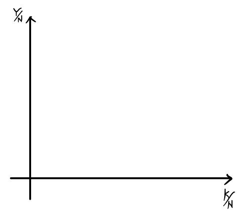
First,

on these coordinate axes,

let’s plot these three things one by one.

In the previous post

we already drew this, right?

Huh??

That, and

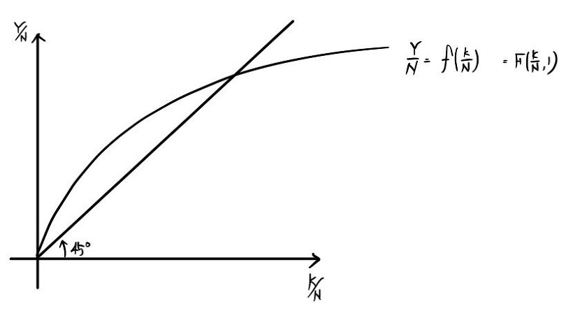
this — they’re the same thing, so we just draw it the same way we drew it last time.

I drew it the same as before, auxiliary lines tossed in and all!!

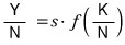
Next thing we also have to draw is

this — but the savings coefficient $s$ is a number with $0 < s < 1$, right?

So each point lands at a spot where the function value above gets knocked down by $s$%!!!

And the reason I drew the auxiliary line at 45° on the figure above is

so we could draw this.

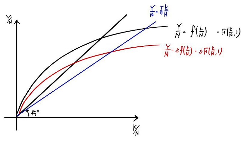
The variable on the $x$-axis is $K/N$. So we can just think of it as

$$y = \delta x$$

and plot it, and since $\delta$ is the depreciation coefficient, it’s also a number between 0 and 1.

So let’s overlay the two functions on the graph above!!

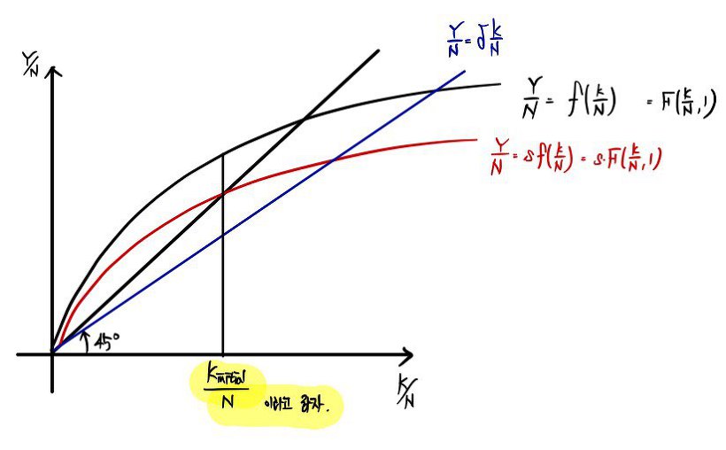
Clear now?!?!

OK now let me bring the equation back in.

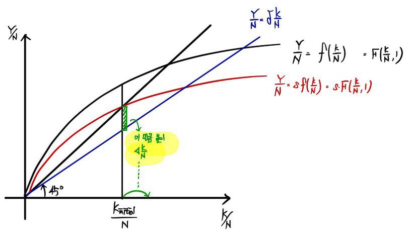
There it is.

The change in capital per person equals the difference between the function value of the red curve and the function value of the blue curve at that spot!!

I said I’d derive the steady state — so let me actually do it.

Let’s drop our initial capital stock right here.

The gap between red’s value and blue’s value at that point — that’s the “change in capital stock”!!

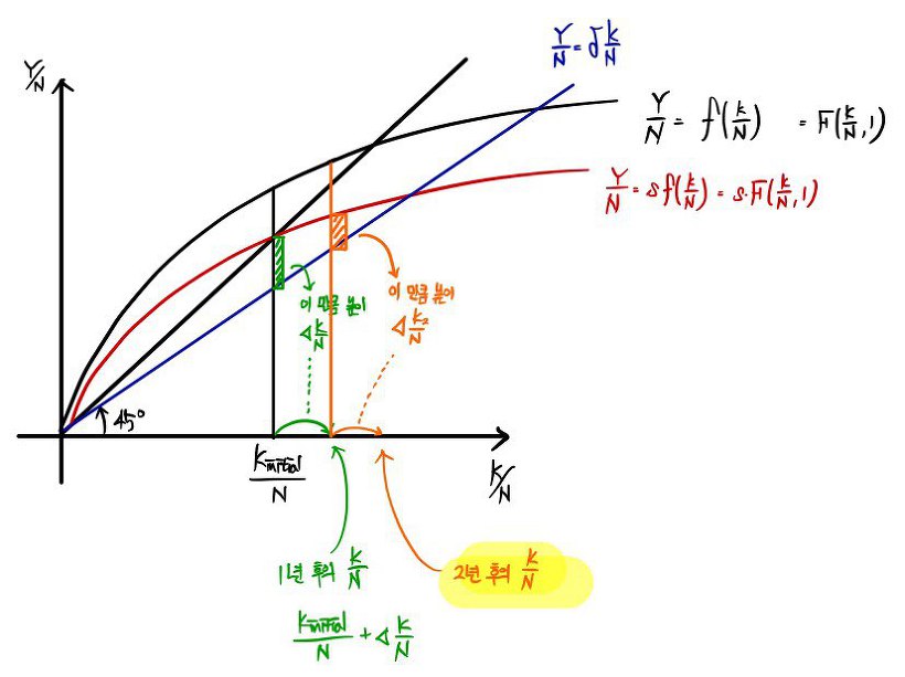
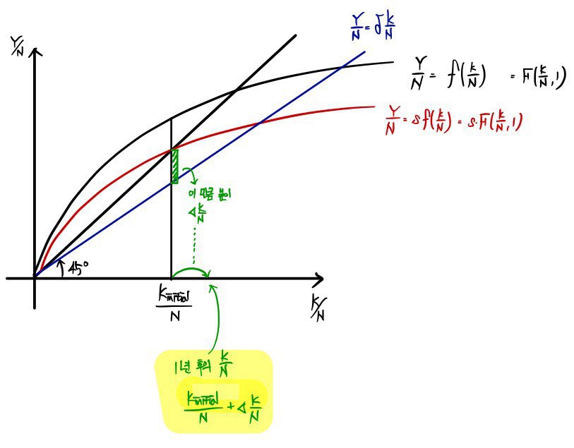
Meaning: capital per person in the following year ticks up from $K_{\text{initial}}/N$ by exactly that red-minus-blue gap.

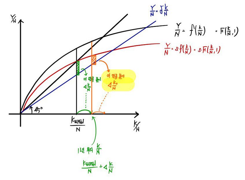
Now the next year arrives. And next year, there’s still a gap between red and blue.

That remaining gap pushes capital up again!!!

By that much, it inches forward once more.

“How long does this whole thing keep happening?????”

Right here, wouldn’t it?

It’d stop right here!!?!?

Because past that point, the gap between red and blue goes negative ($-$), so it comes back. Then the gap is positive ($+$) again, and it gradually gradually gradually gradually creeps toward the intersection of red and blue, and after that it almoooost stops. (More accurate phrasing: it converges to a stop.)

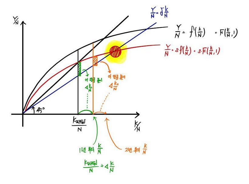
So we can call that arrival point the steady state, right?

Let me mark and write down the ordered pair at that intersection like this:

That point is the steady state.

OK so let me throw out a question.

If the initial amount of savings changes, can the steady-state value of

change??

Absolutely not, right?!

It does not depend on the initial capital stock — what determines it is the savings coefficient $s$ or the depreciation coefficient $\delta$.

More precisely,

this is what determines it.

Aha!!! So the things that determine the steady state are $s$, $f()$, and $\delta$!!!

1. If the savings coefficient $s$ is a bit bigger than before,

gets bigger than before.

2. If the depreciation coefficient $\delta$ is a bit bigger than before,

gets smaller than before.

3. If the level of technology goes up,

gets bigger than before.

So that’s how the steady state shifts as each variable moves~

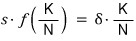
One thing to keep in mind:

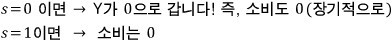
when $s = 1$ — savings-rate-wise — we get the

maximum~~~

Now, something feels weirdly off about that.

If the savings rate is 1, that means people are consuming literally nothing and going all-in on saving — and by doing that, you get the Maximum output achievable under identical economic conditions??

Clearly, to make $Y$ grow overall, “consumption” is also something you can’t just toss out!?!?

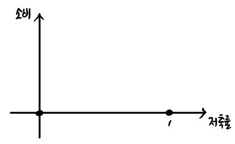
Let’s try two extreme situations.

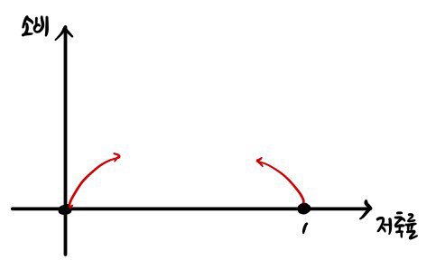
So!!!! when $s$ gets juuust a smidge bigger than 0, $Y$ gradually gradually gradually rises, and through that, consumption rises too.

And when $s$ gets juuust a hair smaller than 1, consumption also juuust slightly creeps up?!?!

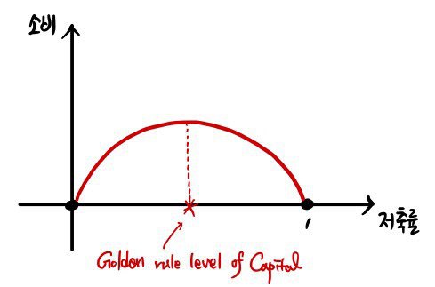
Which means: there’s a savings rate that maximizes consumption at the steady state.

That’s called the golden rule level of capital.

To pin down the exact value, we’d need an equation to differentiate or something.

Right now we don’t have an equation, so… yeah, nothing more we can do here.

Anyway — inside the relationship between the savings rate $s$ and $Y/N$, we slid consumption in and got the mechanism out, apparently.

---

Originally written in Korean on my Naver blog (2016-01). Translated to English for gdpark.blog.