Solow Residual: A Macroeconomic Approach to Technological Progress

So far, the indicator of economic growth we’ve been using is per-capita GDP — Y/N!!!

We said the variables that determine this are K, N, and F(~), and we already chewed on K for a while.

This time, let’s turn our attention to the ’level of technology’ that’s hiding inside F(~).

Just a tiiiny bit more detail than the F(~) we covered before, so don’t get your hopes up too high.

The reason: we’re going to take labor productivity A — which we’d been pinning at 1 the whole time — and let it actually be a variable.

Wait!! Why is A making a comeback here?!

Can we just say labor productivity A represents the level of technology?!

Eh, sure, close enough… (technically they’re different things, but whatever.)

Let’s just go ahead and call A the ‘state of technology.’

We had Y = AN, right??? Plus,

we’d also assumed another variable K that helps determine Y. So the function F that gives Y becomes

$$F(K, AN)$$

— let’s view it like this.

The variables we’re feeding in are K and AN.

The thing I want to emphasize is NOT that A and N are being treated as two separate inputs.

It’s that we’re lumping AN together and treating it as a single variable.

Why does that matter? Saying “the level of technology doubled” means 2AN…

but that’s only the story if the amount of labor N is held constant.

Like, if technology actually advances, are they really gonna leave the headcount alone? Really? Wouldn’t they trim a few people? Come on.

So if you try to think of A and N separately, your head starts to hurt.

That’s why the move is to lump AN together, call it “effective labor,” and keep going from there.

Let’s keep that view and push on.

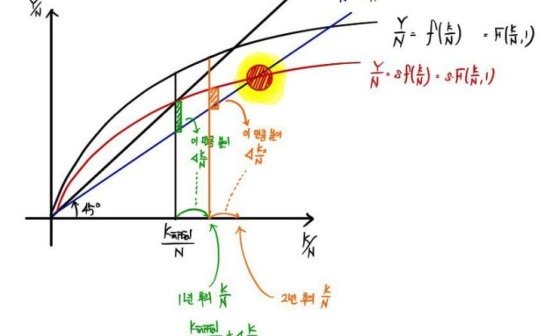
$$\frac{K}{AN}$$

I want to draw this on a coordinate axis.

Now that we’re treating AN as ’effective labor,’ we can apply the exact same logic from Chapter 10 — verbatim.

What was that logic? I’m just going to swap ’labor’ for ’effective labor’ everywhere.

When K = 5 (machines), AN (effective labor) = 5 people,

let’s say Y = 5.

$$Y = F(K, AN) = F(5, 5) = 5$$

But say we bump it up by another 5 machines and another 5 effective labor!!!!

What does output Y become?!?!?!?!?!

$$Y = F(10, 10) = ?$$

Yeah!!! It would double, since we’re producing 5 more of the exact same thing?!?!?!?

Which means our function F has the following property.

This kind of property:

$$F(xK, xAN) = xF(K, AN)$$

We’re going to milk this property.

Let’s plug in x = 1/AN!!!

$$F\!\left(\frac{K}{AN},1\right) = \frac{1}{AN}F(K,AN) = \frac{Y}{AN}$$

That’s what we get.

And to clean up the notation, let

$$f\!\left(\frac{K}{AN}\right) = \frac{Y}{AN}$$

— shorthand it like that.

Then the graph comes out exactly the same shape, right?!?!?! (The shape, anyway. Just the shape.)

OK and now we’ll also need to peek back at the chain of logic we already walked through.

Because the same exact thing applies here.

Under the assumption NX = 0 and T − G = 0, we get I = S.

Savings S is proportional to income Y, and if we call that proportionality constant s, then S = sY,

so I = sY. Tack on a time index and

$$I_t = sY_t$$

we get this.

Now capital K at time t,

$$K_t$$

minus what depreciation eats away,

$$K_t(1-\delta)$$

flows forward,

so capital (flow + stock) at time t+1 becomes

$$K_{t+1} = K_t + I_t - \delta K_t$$$$K_{t+1} = K_t + sY_t - \delta K_t$$

Wow~~~~ we got here through the exact~~~same chain of logic.

OK so in this chapter, we said we’d release the assumption that N is constant.

Why release it? Because we’ve introduced time as a variable, and we need to look at how things evolve as time passes.

We said we’d let A vary because it changes over time —

but it’s also kinda unreasonable to keep N nailed down as a constant,

so while we’re at it, we’re dropping that assumption for N too!~

If A and N both change like that, which part of the equations above do we need to fix? It’s

$$\frac{K_{t+1}}{A_{t+1}N_{t+1}}$$

— that part there in the spotlight.

Capital per unit of effective labor

gets eaten away by the depreciation rate δ, AND on top of that,

$$g_A$$

— the rate of technological progress, and

$$g_N$$

— the rate of population growth. It’ll get knocked down by the sum of those rates.

(Quick example — if depreciation is 10%, the rate of technological progress is 2%, the rate of growth in workers is 1%, then from year t’s capital stock,

$$\delta + g_A + g_N = 13\%$$

gets shaved off, and what’s left flows in as year t+1’s capital stock!!!)

That is,

$$\frac{K_{t+1}}{A_{t+1}N_{t+1}} = \frac{K_t + sY_t - \delta K_t}{A_{t+1}N_{t+1}}$$

— this is the bill we pay for letting those variables roam free!!!!!!!

Let’s call that newly minted total decrease rate Δ!!!

$$\Delta = \delta + g_A + g_N$$

Why bother packing it like this????????????????

So we can run the exact~~~same chain of logic we ran before!! heh heh heh heh heh

Go check the earlier post!!! Linking it ( http://gdpresent.blog.me/220592304061 )

The relationship between the savings rate and output [ My Study of Macroeconomics #11 ]

In the previous post we decided to take the indicator of economic growth as ‘per-capita output’ (if per-capita output goes up, then economic growth…

gdpresent.blog.me

The fact that the conclusion comes out the same means

$$\frac{Y_t}{A_t N_t} = f\!\left(\frac{K_t}{A_t N_t}\right)$$

a steady state exists!

And the value of Y(*) doesn’t depend on the initial capital stock per unit of effective labor!!!

But — there’s a twist this time.

The steady state here is

$$\frac{K^*}{AN}, \quad \frac{Y^*}{AN} = \text{constant}$$

these guys are constant.

But meanwhile, AN itself is changing as time passes.

How is it changing? It’s growing at rate

$$g_A + g_N$$

— this rate.

So back when N was held constant, Y had a hard ceiling, and the rate of change of

$$\frac{Y^*}{N}$$

in the steady state was 0. Here, though, Y and K are both

$$g_A + g_N$$

— changing together at this rate.

Summary:

The rate of economic growth in the steady state is

$$g_A + g_N$$

this.

If

$$g_A + g_N$$

is zero, the rate of economic growth is zero.

In this case, this kind of growth rate is called the “balanced growth rate” —

$$g_A + g_N$$

— that’s it.

OK, before we move on, let’s clear up one nagging question.

$$g_N$$

— the growth rate (or rate of change) of labor — that one doesn’t seem too crazy to pin down with stats from the bureau of statistics or wherever.

But seriously, what on earth is

$$g_A$$

— the rate of technological progress — and how the heck do you put a number on it!!!!

Let me introduce something for that.

There are various ways to quantify it, and among the ones still in active use today,

I’ll introduce Robert Solow’s method from ‘57.

$$Y = F(K, AN)$$

we have this, right?!?!?!

$$\frac{\Delta Y}{Y} = \alpha \frac{\Delta N}{N} + (1-\alpha)\frac{\Delta K}{K} + \frac{\Delta A}{A}$$

To express it as a rate of change,

$$\frac{\Delta Y}{Y}$$

we can shuffle things like this,

and write

$$\frac{\Delta Y}{Y} = \alpha \frac{\Delta N}{N} + (1-\alpha)\frac{\Delta K}{K} + \frac{\Delta A}{A}$$$$\alpha \frac{\Delta N}{N}$$

where α is “the share that wages take of total output.”

So if we call labor’s share α and rewrite,

$$\alpha \frac{\Delta N}{N}$$

is the change in output attributable to changes in labor. (Naturally α is a number between 0 and 1.)

Then there’s gotta be a chunk attributable to capital too, right?

$$(1-\alpha)\frac{\Delta K}{K}$$

We take these two measurable things and subtract them

from the actually measured

$$\frac{\Delta Y}{Y}.$$

And whaddya know — there’s a leftover!!!!!

So

$$\frac{\Delta A}{A} = \frac{\Delta Y}{Y} - \alpha\frac{\Delta N}{N} - (1-\alpha)\frac{\Delta K}{K}$$

— this is called the Solow Residual.

Why does the residual show up? Probably because of technological progress.

Going with that thought,

it seems fair to label that residual

$$\frac{\Delta A}{A}$$

— yeah, that works!!!!!

BUT!!!!! No matter how juicy the tech is, if there’s no labor around, technological progress is completely useless.

$$g_A = \frac{\Delta A}{A} \cdot \frac{1}{N}$$

is how it’s defined, apparently^^

Not too gnarly a concept.

---

Originally written in Korean on my Naver blog (2016-01). Translated to English for gdpark.blog.