Compensating Variation and Equivalent Variation

So far we’ve been hyper-focused on which x gets picked.

This time? I want to zoom in on utility instead.

Let me start with something we already know in our bones — common-sense stuff.

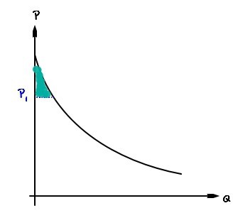
When you’ve got a demand curve like this, the area underneath it is the consumer’s utility.

We call this guy consumer surplus.

So when the price is $P_1$, the consumer surplus (a.k.a. utility) is exactly that shaded chunk up there.

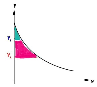
Now drop the price down to $P_2$ — consumer surplus grows by the red bit.

In other words: price falls from $P_1$ to $P_2$, and the increase in consumer surplus (utility) is the red region.

Which means total consumer surplus at $P_2$ is blue + red.

This is the kind of thing they hit you with around Intro to Econ, right?????

Mankiw covers it in like one neat little box. Easy.

OK — now this ‘increase / decrease’ in utility — this time around,

we want to look at it on a coordinate-axes graph like this one.

Obviously,

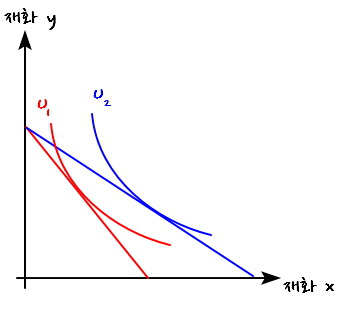
when the price of x drops from $P_1$ to $P_2$, utility

clearly jumps from $U_1$ to $U_2$, right?@??@@?@!!!!

So here’s the question: when it goes from $U_1$ to $U_2$, is that increase

the same as

this guy right here from the demand curve~~~~

That’s what we’re gonna check.

Using what???????????????????

Specifically,

compensating variation & equivalent variation —

those are the concepts we’ll lean on.

Before we get into it, we gotta nail down some definitions first. Let me just slam them down and we’ll move on.

Equivalent variation:

The change in utility caused by a price change —

pretend the price didn’t actually change (keep it at the pre-change price), and pretend instead that income changed —

how much would income have had to go up to give you that same utility change? That amount of Δincome.

Compensating variation:

The change in utility caused by a price change —

now pretend the price is at the post-change price, and pretend income changed —

how much would income have had to go up to give you that same utility change? That amount of Δincome.

OK what on earth is this even saying right now…..

Look — when the price of x falls, the person’s utility went $U_1 \to U_2$, right???

To get that same amount of utility at the original (pre-change) price — how much would income have had to bump up?

In other words: pin the price at the pre-change level, and ask how much income needs to grow so that utility goes $U_1 \to U_2$…

For that to happen,

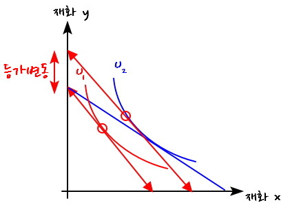
we’d have needed an income jump this big.

That income amount? That’s what we call equivalent variation@@@

(The whole vibe here is: measure a utility change as if it were an income change!!

— makes sense, since the unit of area under the demand curve is also [$] money anyway.)

Same deal for the utility change $U_1 \to U_2$, but this time pin the price at the post-change price for x,

and let’s measure that utility change as income.

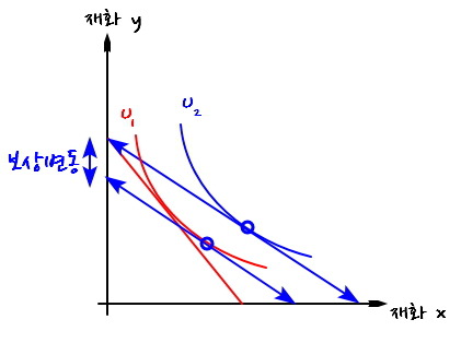
We do that by drawing the blue auxiliary line (locking in the post-change price),

and the income change of that size —

the amount of income that drags utility from $U_1 \to U_2$ — that’s what we call compensating variation.

And now we compare that colored Δconsumer surplus over there

with the CV and EV from above,

and the relationship that’s said to hold is the following.

(Punchline: when there’s an income effect, consumer surplus can’t really be measured properly.)

(Exception: the sign can flip for inferior goods, or when prices rise.)

http://gdpresent.blog.me/220904336701

Microeconomics I Studied #47. Let’s Solve Chapter 5 Problems

The first part was easy so I just threw it up as photos, but from here on I’ll type it out as much as I can …

blog.naver.com

Originally written in Korean on my Naver blog (2016-07). Translated to English for gdpark.blog.