Marginal Rate of Technical Substitution

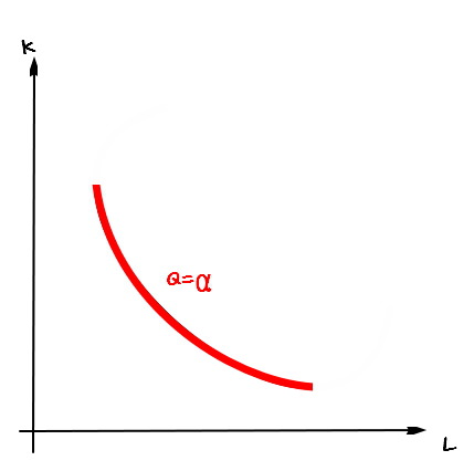
Last time we derived the isoquant graph!!

So once we’ve drawn a graph, what do we always do next???

Right. Same drill here — we need to figure out what the slope means.

Why the slope of an isoquant is a meaningful thing —

once you see the meaning, it’ll click. Trust me.

OK so let’s first nail down what the slope is telling us in this graph.

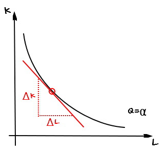
We’re going to work out the meaning of the slope of the tangent line at each point.

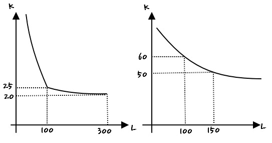
“If I bump $L$ by $\Delta L$ at this point and I still want to produce the same output $\alpha$, how much $\Delta K$ of capital can I get rid of?”

That’s the kind of number we’re looking at.

Or, flipping it around:

After tossing $\Delta L$ of labor, how much extra capital do I need to still pump out the same $Q$????

So the slope of the isoquant

is saying “the rate at which labor and capital can substitute for each other.”

That’s why the slope of the isoquant

gets the fancy name marginal rate of technical substitution of labor (for capital).

The idea is that everything — the machines’ tech, the workers’ know-how, all of it — gets lumped under the word “technology.” So don’t get tripped up by the name.

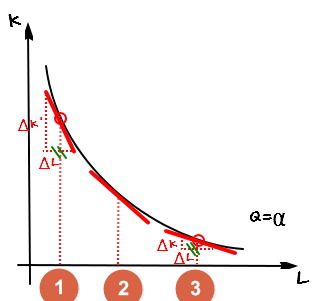
Look at points 1 and 3. Same $\Delta L$ being added, but the amount of $K$ you can throw away — $\Delta K$ — is different.

At point 1, $\Delta K$ is bigger.

And as we slide from 1 toward 3, the $\Delta K$ you can ditch for the same bump in $L$ keeps shrinking.

So the rate at which you can swap out capital for “more technology / labor” gets smaller and smaller.

This is what we call the diminishing marginal rate of technical substitution, heheheh.

OK now — same as we did with the utility curve — let’s write this out mathematically.

What we want is the slope $dK/dL$.

But this curve is an isoquant, which means… it’s the set of points that all share the same $Q$.

And $Q = f(L, K)$,

so it’s a two-variable function in $L$ and $K$,

which means $dQ$ shakes out like this:

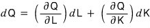
That’s the total differential.

But our concern is “on the isoquant,”

and on the isoquant $dQ = 0$, so:

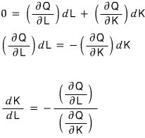
Now, since we want the left-hand side — the slope, our MRTS — to come out as a positive number, we slap a minus sign in:

Alright, now let’s re-read the graph through this MRTS lens.

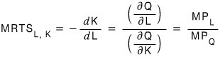
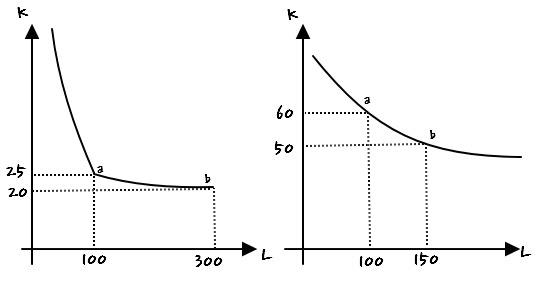
Suppose we have two companies, and their isoquants look like:

Like that.

i) In the left graph, if you want to change $K$ by even a tiiiny~~~ bit, you need a huge change in $L$.

In the right graph, on the other hand, even a moderate change in $K$ doesn’t ask for nearly as big a swing in $L$ as the left one does.

Which company would you want to work at?????

The right one can shuffle $K$ and $L$ around pretty easily.

The left one? Changing $K$ and $L$ is a Big Decision —

not the kind of thing you just casually do.

So: as a worker, you’d pick the left company. As a boss, you’d want to build the right kind of company so the operation runs smooth.

The size of MRTS basically tells you whether you can smoothly tweak your $L$-to-$K$ ratio or not —

that’s how I want you to think about it.

MRTS lives somewhere between $0$ and $\infty$,

and the further it is from $1$ —

whether it’s $10000$ or $1/10000$ — the harder it is to shift the K-L capital ratio @@@@

and the closer MRTS is to $1$, the easier it is to shift the L-K ratio @@

Make sense?~~~

OK so now let’s say we’ve become the boss.

We need to know our company’s isoquant,

and ideally we want our MRTS sitting at $1$.

Because at $1$, whenever some external shock comes flying in,

we can respond by quickly-quickly-quickly-quickly-quickly shifting our $L$ and $K$ ratio.

Let’s say the $Q$ our company is currently producing is

about that much, but I’m not happy with the L&K ratio.

Because MRTS is a bit far from $1$.

So the boss sits there thinking:

“Haaa…. at our current level, what percentage change in $(K/L)$ do I need to lower MRTS by $1\%$?????”

I just sneakily slipped a definition in there.

Which one, you ask —

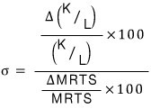
Elasticity of substitution, $\sigma$.

That’s the one.

In formula form:

OK, now let’s go back to that two-companies graph from earlier @@@@@@

and plug in some reasonable numbers and see what falls out.

Starting from the left: moving from point $A$ (where we are now) to point $B$ — what’s the $\%\Delta(K/L)$ we need to change MRTS by $1\%$?!?!!!

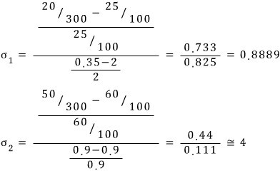
(The MRTS values were given — I just didn’t bother writing them onto the diagram.)

What I wanted to show numerically is this:

when capital and labor are hard to substitute, $\sigma$ is close to $0$,

and when they’re easy to substitute, $\sigma$ can blow up all the way to $\infty$.

Originally written in Korean on my Naver blog (2016-07). Translated to English for gdpark.blog.