Returns to Scale

This time we’re looking at the three-dimensional production function $Q = f(K,L)$ instead of the isoquant.

Let me toss out a question.

Production quantity $Q$ depends on capital $K$ and labor $L$.

Right?!

So here’s the question.

If we crank both $K$ and $L$ up by 2x, does $Q$ also become 2x?!?!?!

Put more simply — if there was 1 factory and now there are 2 factories, does production double?!?!

Feels like it should, right?!?!!!

OK let me rephrase the question.

Samsung’s semiconductor fab in Suwon doubles all its machinery and equipment, and also doubles its labor.

Meanwhile, let’s say Hynix builds a brand new semiconductor fab somewhere else over in Icheon.

Which one ends up with a bigger jump in $Q$?

You’re not gonna tell me both come out to exactly 2x, right????

Obviously, scaling up one existing factory to twice its size is more effective in terms of cost reduction —

i.e. Samsung pulls off bigger cost reduction than Hynix does.

Let’s draw this cost reduction situation on a graph.

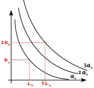
This kind of picture is what successful cost reduction looks like, right?@??@

Ah, OK — now I’m getting the feel for the whole thing.

Looks like we can also draw the break-even case and the case where costs actually got worse.

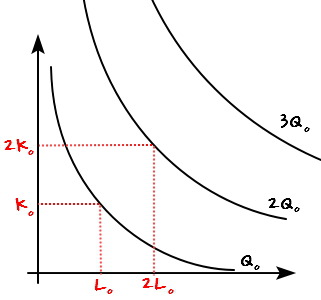
This one’s the break-even picture.

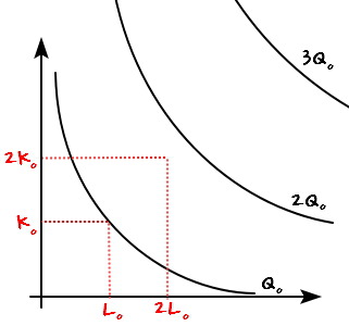
And this one’s the case where you ate even more of a loss.

Where does the cause of all this live…?

Isn’t it efficiency???

Those

,

,

isoquants are curves you get by slicing the 3D production function parallel to the $L$–$K$ plane,

and the reason

,

,

end up packed close together — that’s because of this.

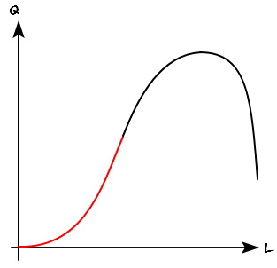
This red part!!!!!

This part where efficiency just keeps rising like crazy@@ Here, even if you cut planes

,

,

perpendicular to the $Q$ axis, they’re gonna be packed in tight.

<Increasing returns to scale>

Then, the failure-at-cost-reduction case is the leftover part on the graph.

In this part,

,

,

are gonna be spread out wide and roomy,

and this is the region where the rate of efficiency increase was gradually slowing down@@@

So everything lines up front-to-back like this!!!!

<Decreasing returns to scale>

Increasing returns to scale, decreasing returns to scale, constant returns to scale —

these all become way easier to talk about if the production function happens to be a Cobb-Douglas production function.

If $L$ and $K$ are just sitting there as a product (whatever the exponents are)

then the discussion gets easy.

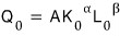
Say the production quantity when the inputs are

,

is

.

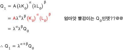
Now, let’s multiply each input by $\lambda$.

Plug in

,

. Call the production quantity at this point

.

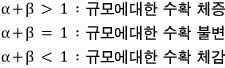
If you’ve got a Cobb-Douglas shape, you can tell — straight from $\alpha$ and $\beta$ alone —

whether returns to scale are increasing, decreasing, or constant.

Ah but — Cobb-Douglas is nice and easy, and because of that exact niceness, it can’t really explain a lot of things.

So in econ lectures they call it the undergrad model.

Apparently — once you’re past the undergrad level, Cobb-Douglas doesn’t get used much~

Originally written in Korean on my Naver blog (2016-07). Translated to English for gdpark.blog.