Labor Demand Curve

Today let’s derive the labor demand curve.

Same principle as deriving the demand curve for good $x$ in demand theory. Should feel familiar.

OK let’s go lol.

So labor demand — from the firm’s side — is basically “how badly does the firm want labor?”

<And of course, the firm will want the $L$ that minimizes cost.>

But there’s a premise hiding in there: “the cost $r$ of capital $K$ is constant.”

And then, depending on the level of $w$, we trace out how the firm’s want-for-labor changes!!!

That’s the labor demand curve!!!

OK OK OK, let me draw the isoquant and isocost first.

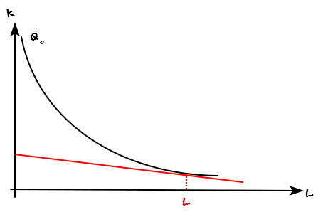
Say the initially-fixed $r$ and $w$ give the isocost line this slope.

Find the $L$ that minimizes cost right now,

and jot the pair down as $(L, w)$.

Now say the wage bumps up a little — call it $w'$.

With $r$ held fixed and $w \to w'$, the isocost slope becomes

$$-\frac{w'}{r}$$

which is smaller than the previous slope. Steeper, in other words.

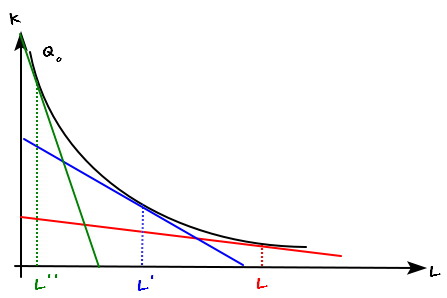
So the isocost tilts to this new slope, and we look for the $L'$ that minimizes cost while still producing

$$Q_{0}$$

and write down $(L', w')$.

Bump the wage again, $w' \to w''$, isocost gets even steeper, find the labor $L''$ that minimizes cost at that point, jot down $(L'', w'')$ too.

Now imagine we repeated this infinitely many times. For an ever~~~so tiny change $dw$, we figure out what the tiny corresponding $dL$ is.

Take all that extracted info and —

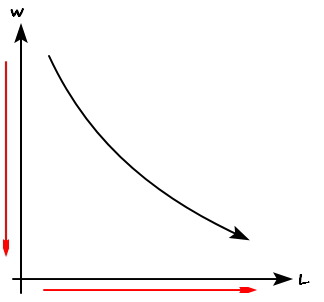
— plot it on this $w$-$L$ axis, in the direction where as $w$ goes up, $L$ goes down.

Hmm…..

Saying “as $w$ goes down, $L$ goes up” is the exact same thing anyway, so on the axis above, let’s just draw it that way — $w$ falling, $L$ rising.

There. That’s how you’d draw it.

Don’t believe me?

OK fine, let me derive it properly with math too.

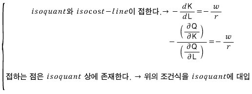
I want to derive it from these two pieces of logic, but I don’t have a convenient production function lying around.

So let’s just assume the isoquant comes from a generic Cobb-Douglas, and follow the logic above:

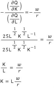
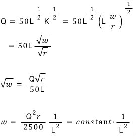
$$Q\quad =\quad 50L^{\frac{1}{2}}K^{\frac{1}{2}}$$

Cool. Then condition 1 above becomes —

And condition 2 applied to condition 1 means plugging condition 1’s equation into the isoquant. That is,

We already agreed $Q$, $r$, all that — they’re constants. So the final form pops out looking like that.

And see? Just like that, we’ve got a relationship between $w$ and $L$.

So now,

you’ve got a rough feel for why the labor demand curve gets drawn like this, right~~~

OK then —

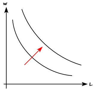
$$w\quad =\quad \frac{Q^{2}r}{2500}\frac{1}{L^{2}}$$

— eyeballing this shape: if the firm decides to crank $Q$ up, how does the labor demand curve change???

Something like this, right??? (and it will absolutely not be a parallel shift)

At least under Cobb-Douglas, that’s how the labor demand curve responds to changes in $Q$.

Oh@ — one more thing to watch for.

Like, when some firm tries to ramp up its output, does it necessarily want more labor?????

Nope. Not always.

For firms where “labor” as a factor of production is a normal input, sure, yeah.

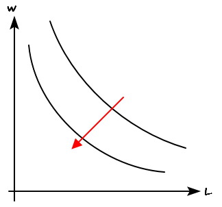
But for firms where labor is an inferior input, cranking $Q$ up can actually decrease $L$.

That is,

if you see a labor demand curve shift like this when output goes up — nothing weird about it at all, is what I’m saying.

We just shrug and go “ah right, so for you guys, labor’s an inferior input^^*”

---

Originally written in Korean on my Naver blog (2016-07). Translated to English for gdpark.blog.