Short-Run Analysis

Alright, long run’s done. Time for the short run.

Remember way back at the start — the difference between long run and short run isn’t really about time. It’s about flexibility. Total flexibility = long run. Some things locked in = short run. That’s the whole distinction.

Which means: in the short run, total cost picks up a new component that didn’t exist in the long run. A fixed cost.

So now,

Total cost = variable cost + fixed cost.

In the long run, under our running assumption that total cost is pinned down by $L$ and $K$, we had:

$$TC \quad = \quad wL \quad + \quad rK$$

In the short run, we add one more assumption: $K$ can’t change.

The intuition is what you’d expect:

“You can’t shut down a factory overnight and liquidate it, can you?” “You can’t fire your full-time employees tomorrow, can you?”

That kind of vibe.

OK so from here on, let’s lock $K$ at the constant $\overline{K}$, and let $L$ stay free as the variable input. (We need something to play with, otherwise there’s nothing to discuss!!)

$K$ being fixed at $\overline{K}$ means: “in the short run, you can’t adjust your capital. Even if you produce nothing, the factory’s still there, the interest on the loan you took out to build it is still ticking… etc.” — all of that gets captured as fixed cost.

Now let’s see how to minimize cost when $K$ in total cost is locked at $\overline{K}$. Super simple. First, suppose $w$ and $r$ are already pinned down, and the firm wants to produce a quantity $Q_{0}$.

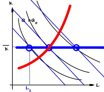
We want to produce this $Q_{0}$, and let’s say the fixed $\overline{K}$ is sitting somewhere around there.

$w$ and $r$ are set, so when we draw an isocost line with slope $-\frac{w}{r}$, the cost-minimizing point would be —

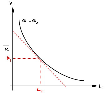
— right here, inputting $(L_{1},\quad K_{1})$. That’d be ideal! Except… our $K$ is locked at $\overline{K}$, so we can’t use $K_{1}$… T_T

So, to produce $Q_{0}$ while being forced to use $\overline{K}$,,,,,

the cost-minimizing point under that constraint is:

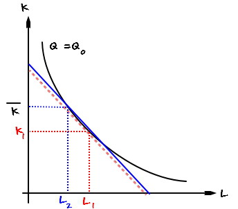
We have to use $(\quad L_{2},\quad \overline{K}\quad)$, sitting on an isocost line that costs a bit more, just to hit $Q_{0}$.

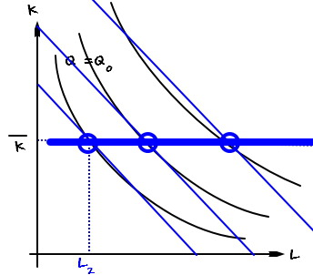
So in the short run, the expansion path looks different from the long-run one. Even as $Q$ increases, $K$ has to stay nailed down at $\overline{K}$. So:

$Q$ goes up, $K$ doesn’t budge. The expansion path ends up looking like this:

Right?!?!?!?!??

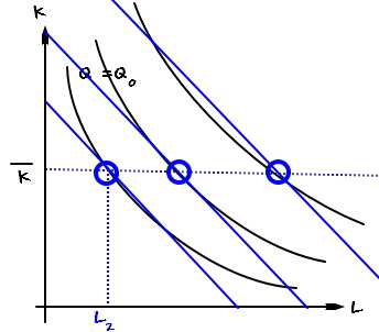
OK hold up — let’s pause and put the long-run and short-run expansion paths on the same axes, shall we?!?!?!??! I’ll just slap the long-run expansion path from earlier right on top.

Like this — and you can see there’s an intersection point between the long-run and short-run expansion paths. And the meaning of that intersection? It’s the $(L, K)$ that minimizes cost — efficiently — in both the long run AND the short run!!!!!

We’ll be hunting for this point in practice problems~

---

Originally written in Korean on my Naver blog (2016-07). Translated to English for gdpark.blog.