Untitled

Last time we cracked open TC, AC, and MC.

That was kind of the big-picture sweep — a general look at how these things show up in the wild as social/economic phenomena, right???

OK, now let’s actually pin them down with something concrete. Cobb-Douglas, undergrad flavor — that’s our production function for today.

Specifically:

$$Q = 50L^{\frac{1}{2}}K^{\frac{1}{2}}$$

First thing we want: as $Q$ goes up, what’s the minimum TC at each $Q$?

Total cost is just

$$TC = wL + rK$$

Yeah, that’s nothing — that’s just the total cost equation. What we actually want is the (minimum) TC as a function of $Q$. heh.

So let’s start with the tangency condition.

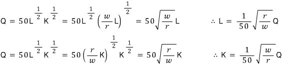
The two gradient vectors have to be parallel, so

And what falls out of this is

$$rK = wL$$

Now — this condition, where does it actually live???

It has to live on the isoquant. So plug it back into the isoquant:

Which means TC is

$$TC = wL + rK$$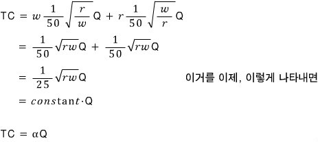

So the TC function for the Cobb-Douglas model is

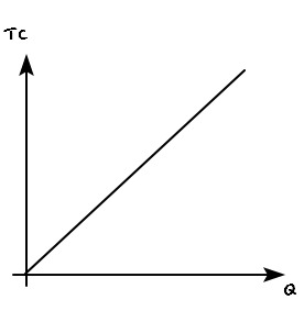
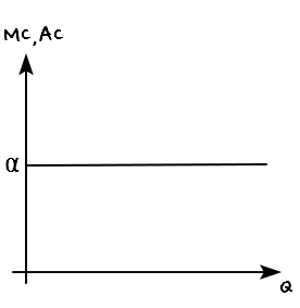
And once TC looks like that, MC and AC fall out in the exact same shape.

The slope of the tangent line at every single point: all α. The slope from the origin at every single point: also all α.

Wait — that’s pretty different from what we had before?!?!?1!!!

Why does it come out like this?

My hunch: it’s because the Cobb-Douglas we’re using here is constant returns to scale. That’s gotta be it.

---

Originally written in Korean on my Naver blog (2016-07). Translated to English for gdpark.blog.