Short-Run Supply Curve (Part 2)

Alright, this time let’s split fixed costs into sunk and non-sunk, and see what happens!

For now, let me drag SAC, SMC, and AVC back onto the board.

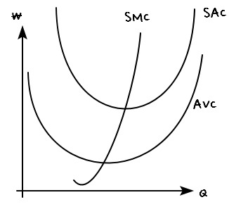
Yeah — not a whole lot is different from last time.

The one twist: among the “fixed costs” filling the gap between SAC and AVC, some of them are non-sunk. That’s the new thing.

OK so the question we need to ask:

Is AVC a sunk cost?? Or non-sunk???

Answer: variable costs are non-sunk too.

Because when $Q = 0$, you can recover them, right????

So let’s chop total cost up into sunk and non-sunk:

Total cost = fixed cost + variable cost

= sunk fixed cost + non-sunk fixed cost + variable cost

= sunk + non-sunk

That’s the split.

Now derive the average non-sunk cost:

Average cost (AC) = average sunk cost + average non-sunk cost (ANSC: average nonsunk cost)

So average non-sunk cost = average cost − average sunk cost.

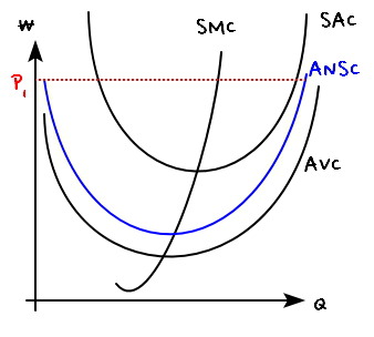
Let’s shade the average non-sunk cost onto the graph above. The move: take SAC, subtract average sunk cost off of it,

and if you draw that on the same graph, you get this:

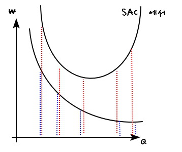
For each $Q$, just subtract the blue from the red, and roughly —

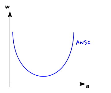
— it’ll come out looking like this.

So if we drop that onto the very first graph,

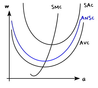
yeah, looks roughly like that.

OK now let’s think about the short-run supply curve in this setup.

First, the case where $P = P_1$, set like this:

The firm, trying to max profit, picks the $Q$ where $P = \text{MC}$, shown below:

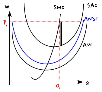
Profit per unit = the ‘black’ amount.

Now the case where price comes in at $P_2$:

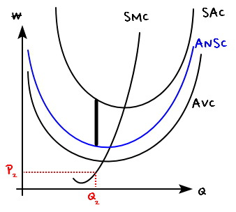
The firm picks $Q_2$ at $P = \text{MC}$ to max profit, and the loss is the ‘black’ amount per unit.

But — if it just doesn’t produce, the non-sunk portion gets recovered, so the no-production loss shrinks to the black amount per unit, and ultimately the firm bails on producing, and the loss sits at black!!!

(Focus on this: no production happens!)

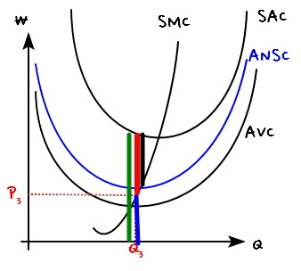
Let’s look at $P = P_3$ now!!!@@@

(Want me to walk this one a bit slower?)

At this price, the firm again picks $Q_3$ as its output — the $Q$ that makes $\text{MC} = P$ — to max profit, and if it goes ahead and produces, the cost per unit is the ‘green’ amount.

But the money it pulls in per unit is the ‘blue’ amount,

so the loss per unit is the ‘red’ amount.

However — if it just bails and doesn’t produce, it recovers the non-sunk costs, and the loss shrinks to the leftover ‘black’ amount per unit!!!!

So this case too, better not to produce. (heh)

Finally, $P = P_4$.

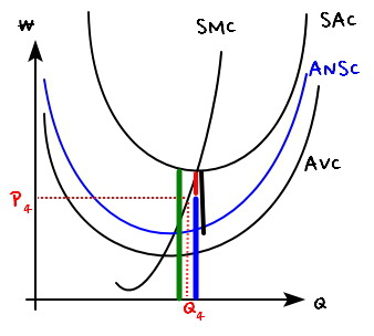
Again, the firm picks $Q_4$ where $P = \text{MC}$.

That is, the firm’s loss is

cost to produce per unit (green) − money received per unit (blue) = (red).

But if the firm, because it’s eating a loss, goes ahead and doesn’t produce, the loss becomes the ‘black’ amount.

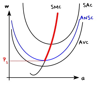
So the conclusion:

the range where $\text{ANSC} < \text{SMC}$ becomes the “short-run supply curve.”

Ah, so when non-sunk costs are baked in among the fixed costs, the shutdown price isn’t

the point where AVC is minimized —

it’s the point where ANSC is minimized. That’s the shutdown price.

Got it sorted? Moving on.

(Short-run supply curve)

Originally written in Korean on my Naver blog (2016-07). Translated to English for gdpark.blog.