Chapter 5 Practice Problems [Microeconomics I Studied #47]

The early problems were easy enough that I just slapped photos in and breezed through them,

but from here on out I’ll try to actually type things out as much as I can.

T_T T_T T_T pleeeease just let me get through this lol lol lol

Prob 5.7

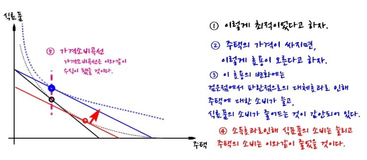
Reggie only consumes two goods: food and housing.

On a graph with housing on the x-axis and food on the y-axis,

the price-consumption curve for housing comes out as a vertical line.

Draw a budget line and indifference curves that are consistent with these preferences.

For reference — a good whose consumption drops because of the income effect is called an inferior good,

and a good whose consumption rises from the substitution effect

but then gets clobbered in the negative direction by the income effect by more than that amount is what we specifically call a GIFFEN GOOD.

Prob 5.8

Ginger’s utility function is

$$U = x^{2}y$$

So the marginal utilities are

$$MU_{x} = 2xy$$

and

$$MU_{y} = x^{2}$$

Income is $I = 240$ and the prices are

$$p_{x} = 8$$

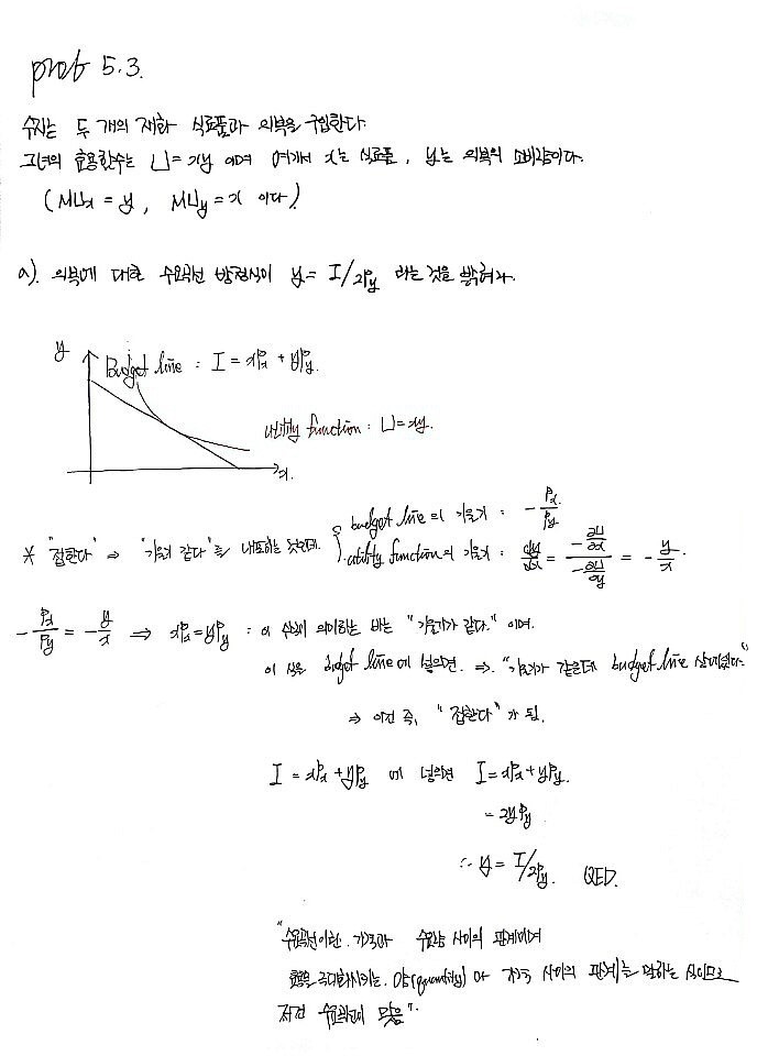
$$p_{y} = 2$$

a) Given these prices and this income, find Ginger’s optimal basket.

At the tangency point, the slope of the budget line equals the slope of the indifference curve, so —

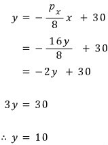
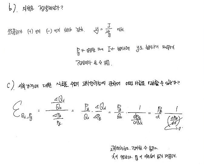
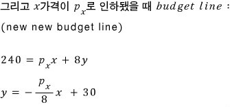
b) If $p_y$ rises to $8 and Ginger’s income stays the same, how low does $p_x$ have to drop for her to keep the same level of welfare she had before $p_y$ changed?

In one sentence, here’s the problem:

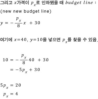
What we’ve been doing all along — we just take that tangency condition and plug it into the new-new budget line, same trick as before.

Because we want to find the spot where the indifference curve from the utility function and the new-new budget line are tangent.

For utility to stay exactly the same, we need to find the partner of $y=10$ that gives us $U = 16000$.

Prob 5.11

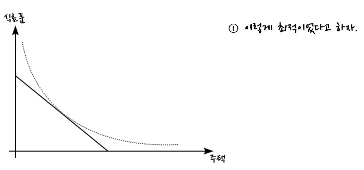
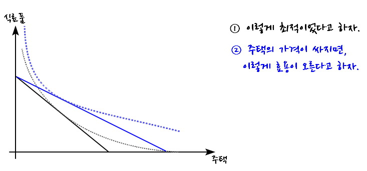
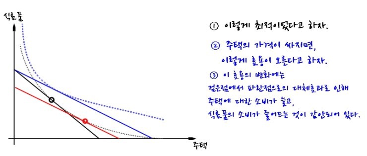
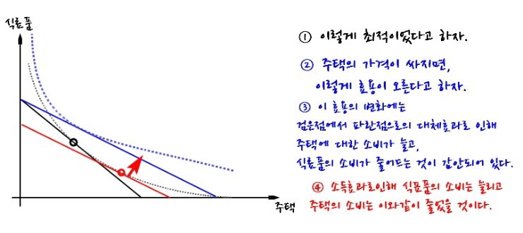
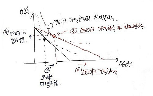
Scott only consumes two goods, steak and ale.

When the price of steak drops, he ends up buying more of both steak and ale.

Explain this with budget lines and indifference curves.

It’ll help if you walk through it in numerical order.

The problem just asks for an explanation, so honestly I think this one diagram is enough.

Prob 5.13

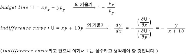
Suppose the consumer’s utility function is

$$U = xy + 10y$$

(This is obvious from a partial derivative, but anyway —)

$$MU_{x} = y$$

$$MU_{y} = x + 10$$

The price of x is $p_x$, the price of y is $p_y$,

both prices are positive. Income is $I$.

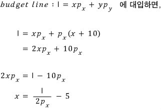
a) Show that the demand for x can be written as

$$x = \frac{I}{2p_{x}} - 5$$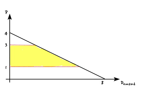

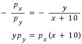
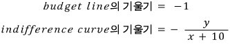
The tangency condition (slopes equal) is

Plug that into the budget line —

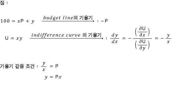
QED.

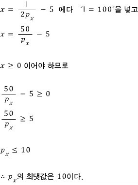
b) Now suppose $I = 100$. What’s the maximum value of $p_x$?

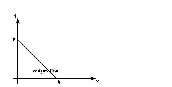
c) Suppose $p_x = 20$ and $p_y = 20$ as well. On a graph showing the optimal basket of x and y, show that since $p_x$ exceeds the value from (b), this is a corner solution where the consumer only buys y.

If $p_x$ and $p_y$ are both 20 and income is 100,

then $100 = 20x + 20y$ is the budget line, so the picture looks like this, right?

Now let’s try to find the optimal point (the one that maxes out utility) using $U = xy + 10y$.

We get $x = -2.5$ —

meaning the x-coordinate of the optimal point is $-2.5$ (and $y$ falls out automatically too — $y = 7.5$).

What this is telling us is —

if we mark the optimal point on the budget line above

OK the indifference curve doesn’t really matter here, I just sketched it however,

but anyway the optimum sits on the budget line at $x = -2.5$ —

right there is where you’d hit max utility.

But hang on — the domain of x doesn’t allow $x < 0$, the negative region.

(We said x is a good being consumed, so negative consumption is weird. It doesn’t even mean selling the good or anything.)

So this consumer, trying to max utility “as best as possible,”

settling for slightly lower utility than the unconstrained max, getting the highest utility you can within the constraint —

— is going to pick $x = 0$. That’s what I’m saying.

So they pick $x = 0$, $y = 5$,

and the utility from that choice is

$U = xy + 10y = 0 \times 5 + 10 \times 5 = 50$.

d) Easy, skip.

e) Still assuming income is 100, draw the demand for x across all values of $p_x$.

The tangency condition is still the same —

Prob 5.15

The demand for some little component is $D = 16 - 2P$.

Calculate the change in consumer surplus when the price rises from $1 to $3.

First, let me sketch the function out a bit.

I’m going to put $P$ on the y-axis and $D$ on the x-axis.

So instead of writing $D = 16 - 2P$,

it’s nicer to write

$P = -(1/2)D + 8$

and draw a line with slope $-1/2$ and y-intercept 8.

OK drawing —

That’s what it looks like, right?

We were asked for the change in consumer surplus when price moves from $1 to $3,

so we need —

— the area in here, right????????

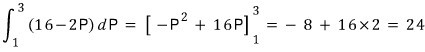
Of course, this area is trivial to compute using right-triangle geometry,

but I’m gonna write it out the hard way for no particular reason.

Why? Just to show it can always be calculated no matter what shape the demand function takes.

The area is 24, and since price went up, utility must have gone down,

and the amount it dropped by is 24,

so $\Delta \text{utility} = -24$.

That’s how I’d write it.

Prob 5.20

Two consumers in the market. (Jim & Donna.)

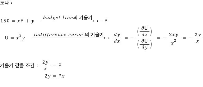
Jim’s utility function is $U = xy$,

Donna’s is $U = x^2 y$.

Jim’s income is

$$I_{J} = 100$$

and Donna’s income is

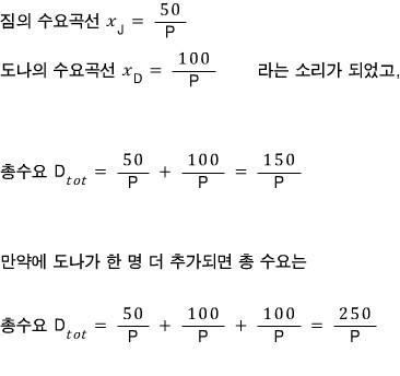
$$I_{D} = 150$$

a) When $p_y = 1$ and $p_x = P$, find Jim’s and Donna’s optimal baskets.

This basically takes us all the way through (d) too.

Prob 5.22

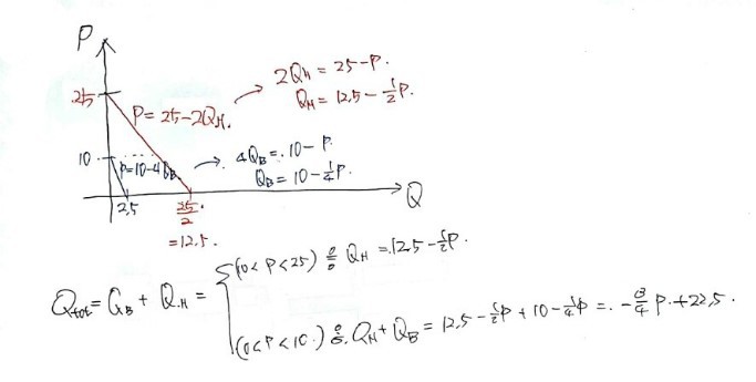
Suppose Bart and Homer are the only people in Springfield who drink the flat soda Seven-Up.

And suppose their respective inverse demand curves for Seven-Up are

$$P = 10 - 4Q_{B}$$$$P = 25 - 2Q_{H}$$

and obviously they don’t consume negative quantities.

Draw the market demand curve for Seven-Up in Springfield.

Oh, this is just asking us to draw two functions

and then draw a new function that’s the sum of the two.

Easy, let’s bang it out and move on.

We just add them range by range,

and the reason the ranges naturally split up is — because the slopes are different, right?

So at the boundary you’ll get a kink. heh heh heh

Prob 5.17

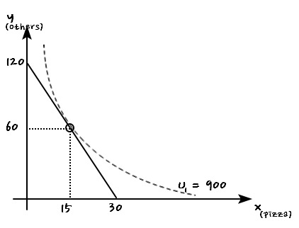
Lou’s preferences over pizza (x) and other goods (y) can be written as $U(x,y) = xy$,

income is 120.

a) When $p_x = 4$ and $p_y = 1$, find the optimal basket.

Ahh, I’m getting kind of sick of these by now….

That’s the condition for the point where the slopes are equal,

and now we plug that into the budget line again.

Let’s plug.

I didn’t bother writing the budget line out above and just said the slope was $-4$ —

because I was saving it for here. That’s why I skipped it earlier.

Anyway, writing it now —

Now let me draw out the situation up to this point.

And then we move on to part (b).

The reason I drew that picture is so part (b) goes nice and smooth~.

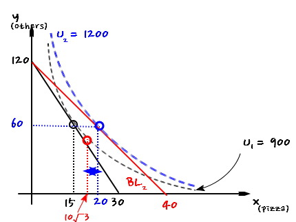
b) When the pizza price drops to $3, calculate the income and substitution effects.

That’s the problem — but on top of income and substitution effects,

let’s go ahead and grab the equivalent variation and compensating variation while we’re at it.

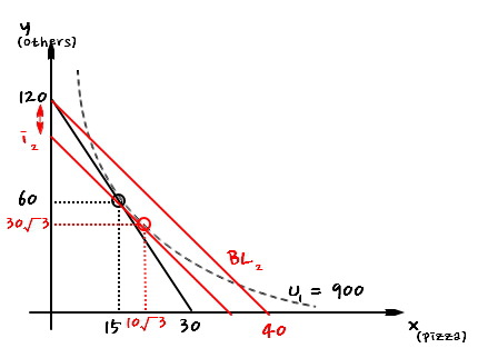
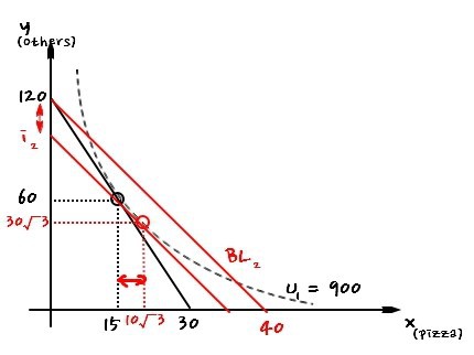
First, since the price moved from $4 to $3,

the new budget line gets drawn in red like this.

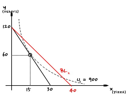
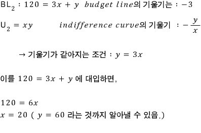
Since $120 = 3x + y$,

the slope of $BL_2$ is $-3$.

OK, let’s first find the compensating variation.

The slope of $BL_2$ is given, and the income is an unknown

$i_2$.

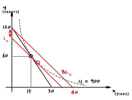
The amount marked by the red double-headed arrow is going to be the “compensating variation” —

the key with compensating variation was “assuming the changed price,” right.

I’m going to find the size of that arrow.

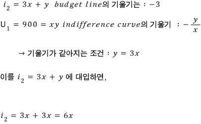
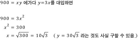
I need to find $x$, and I’ll grab it off the $U_1$ indifference curve.

Because right now $i_2$ is unknown and $U_1$ is known,

instead of plugging the tangency condition into the budget line like we’ve been doing all along,

we plug it into the utility function instead.

(And conversely — the reason we’ve been so casually plugging into the budget line up until now was because income was known and utility was unknown.)

So on the $U_1$ indifference curve, let’s find the $x$ where the slope is $-3$.

Plugging that back into the equation above —

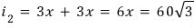
So the compensating variation is

$$120 - 60\sqrt{3}$$

Let me mark all this on the diagram and keep going.

Still with me?

Ah ah ah ah and the red arrow I marked in the figure above —

that amount is exactly the $\Delta x$ from the substitution effect!?!?!?!?!?

That is,

$$\text{Substitution effect} : \Delta x = 10\sqrt{3} - 15$$

Now let’s go find $U_2$.

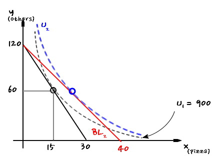
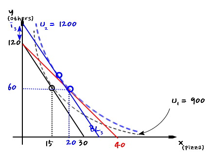
We’re after the $U_2$ that looks like this —

the $U_2$ that’s tangent to $BL_2$ and gives max utility!!!!!!!!!!!!!!!!!!!

Whoa whoa whoa.

So $U_2 = 1200$ is what we calculate.

Then back to the diagram, go go go go go.

Let me re-mark all the info we’ve found.

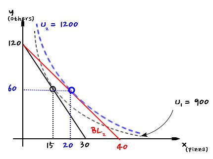
Looks like the income effect is basically locked in now.

Earlier we set the substitution effect as

$$\Delta x = 10\sqrt{3} - 15$$

and from there, the chunk that brought us up to $x = 20$ right now is exactly the income effect.

So —

That amount right there is the income effect.

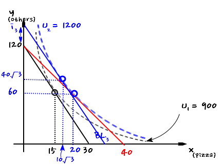
$$\text{Income effect} : \Delta x = 20 - 10\sqrt{3}$$

Now finally all that’s left is the equivalent variation, right????????

Equivalent variation………..

The key with equivalent variation was “assuming the price before the change.”

Let’s keep adding to the diagram.

Assuming the pre-change price,

we need to find the unknown $i_3$.

So I named the budget line with $i_3$ as $BL_3$.

“$BL_3$ — the one with a tangency point like that.”

Then on with the game of hunting down $i_3$.

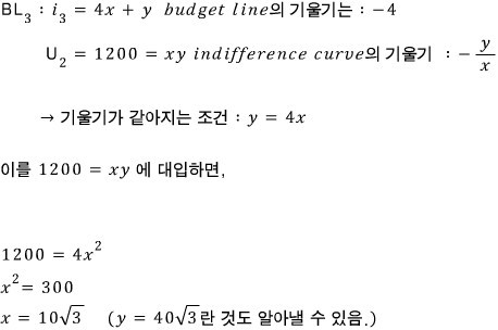
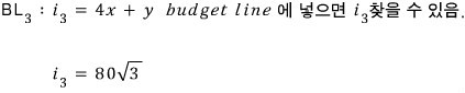
So the equivalent variation is

$$80\sqrt{3} - 120$$

Originally written in Korean on my Naver blog (2017-01). Translated to English for gdpark.blog.