Chapter 6 Practice Problems

Prob 6.3

Production function:

$$Q \quad = \quad 6L^{2} \quad - \quad L^{3}$$

Fill in the table below, then figure out how much the firm has to produce to make each of these happen.

L	Q
0
1
2
3
4
5
6

a) Average product is maximized. b) Marginal product is maximized. c) Total product is maximized. d) Average product becomes 0.

OK, table first!

L	Q
0	0
1	5
2	16
3	27
4	32
5	25
6	0

Just plug into

$$Q \quad = \quad 6L^{2} \quad - \quad L^{3}$$

and read off the values. Easy.

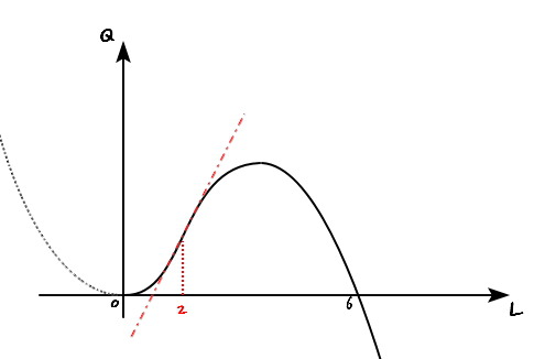
Now to actually solve this stuff, let’s draw the function!!!! I’m gonna draw it the same way I learned in high school, heh.

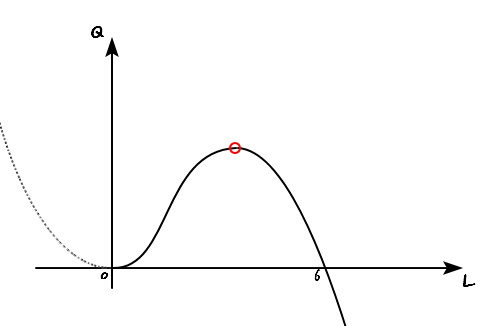
$$Q \quad = \quad 6L^{2} \quad - \quad L^{3} \quad = \quad -L^{2}\left( L \quad - \quad 6 \right)$$

Bounces off at $L = 0$, crosses through $L = 6$, and shoots off to $-\infty$ as $L \to \infty$! hahaha

Ahh but — the region $L < 0$ makes zero economic sense, so we don’t need it on this graph. Erasing it.

Alright~

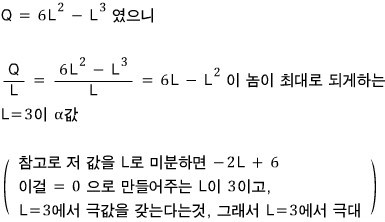
Solving a): “average product is maximized” means we need the value of L that maximizes the slope from the origin.

We’re hunting for the $L = \alpha$ that makes that slope-from-the-origin the biggest.

Concretely, that $\alpha$ is

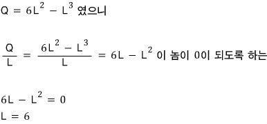
Let’s knock out d) while we’re at it.

When the average product hits 0:

You can do it like that, or you can just look at the graph and find the point where the slope from the origin goes to 0. Same thing.

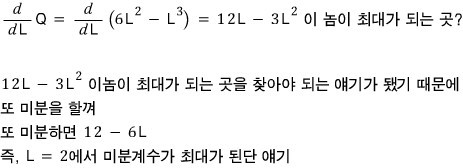
b) asked when the marginal product is biggest, which means: find the point on the graph where the slope of the tangent line (i.e., the derivative) is maximized. In formula form first:

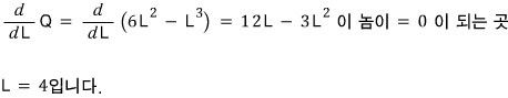
And what does this look like as a picture?

It hits its max right there!!! heh

The last part c) is just finding where Q itself is maximized on that graph above, so

Nothing more than finding the extreme value. $L = 4$.

Prob 6.4

Suppose the production function for DVDs looks like this:

$$Q \quad = \quad KL^{2} \quad - \quad L^{3}$$

Here Q is annual disc production, K is capital measured in machine-hours of input, and L is labor-hours of input — the labor flow.

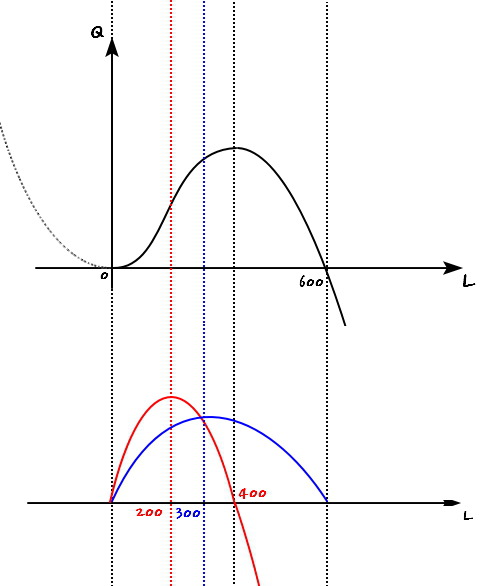
a) Suppose $K = 600$. Find the total product function, plot it over $L = 0$ to $L = 500$, and also draw the average product and marginal product curves. At what level of L does the average product curve hit its max? At what level does the curve hit its max?

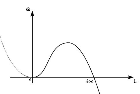
Looks like the move here is just to plug in $K = 600$ and draw.

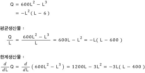
$$Q \quad = \quad 600L^{2} \quad - \quad L^{3} \quad = \quad -L^{2}\left( \quad L \quad - \quad 600 \quad \right)$$

Yep! Recycling the previous shape~

Done!

Now I need MP and AP, so let me grind out the formulas first and then draw.

Based on those, let me also draw the derivative curves. I’ll throw MP and AP on the same picture in one go.

I really should’ve just plotted this with code… I drew it by hand and the scale is off — 300 should sit right at the halfway point of 600, but it doesn’t (T_T). Whatever!!!! You can still tell what’s going on. Moving on.

Prob 6.14

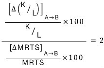
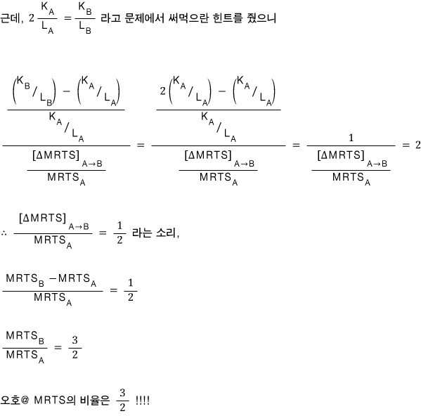
Points A and B sit on an isoquant curve, with labor on the horizontal axis and capital on the vertical. The capital-labor ratio at B is twice the one at A, and as you move from A to B the elasticity of substitution is 2. What’s the ratio of MRTS at A to MRTS at B?

I drew a picture for the vibe, but honestly the problem doesn’t really need it.

That’s the definition, and we were told

$$\sigma_{A\to B} \quad = \quad 2$$

so that means

which gives us

Prob 6.21

Consider this CES (constant elasticity of substitution) production function:

$$Q \quad = \quad \left( \quad K^{\frac{1}{2}} \quad + \quad L^{\frac{1}{2}} \right)^{2}$$

a) What’s the elasticity of substitution of this production function? b) Does it exhibit increasing, constant, or decreasing returns to scale? c) Suppose instead the production function is

$$Q \quad = \quad \left( \quad 100 \quad + \quad K^{\frac{1}{2}} \quad + \quad L^{\frac{1}{2}} \right)^{2}$$

Does this one exhibit decreasing, increasing, or constant returns to scale?

Before diving in, let me throw down the definition of the CES function — which, fair warning, is a little bewildering.

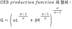
Literally a production function whose elasticity is constant — and presumably this thing was conceived and engineered so that the elasticity comes out constant. How on earth do you cook something like this up??????????????????? I asked this once, and the answer I got was something like: “Well, you’d only really deserve to be called an economist if you could come up with stuff like this,” “and this is the problem with our country’s education system, and this is the problem, and also this is the problem,” “I hope we become a nation that can produce that kind of creative work~” — so I walked away having gotten an earful about the education system hahahaha. Anyway: apparently this is a function dreamed up by someone’s creativity. There’s a ton to say about it in relation to the Cobb-Douglas production function, but I’m not going to dive into the economic significance here — I’ll just solve the problem and bounce.

a) let’s go let’s go let’s go let’s go

Since we’re told it’s a CES production function, looks like we can just pattern-match and read off $\sigma$.

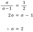
Easy.

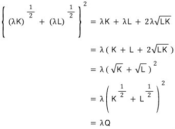
b) Let’s plug L and K each scaled by $\lambda$ and see what pops out.

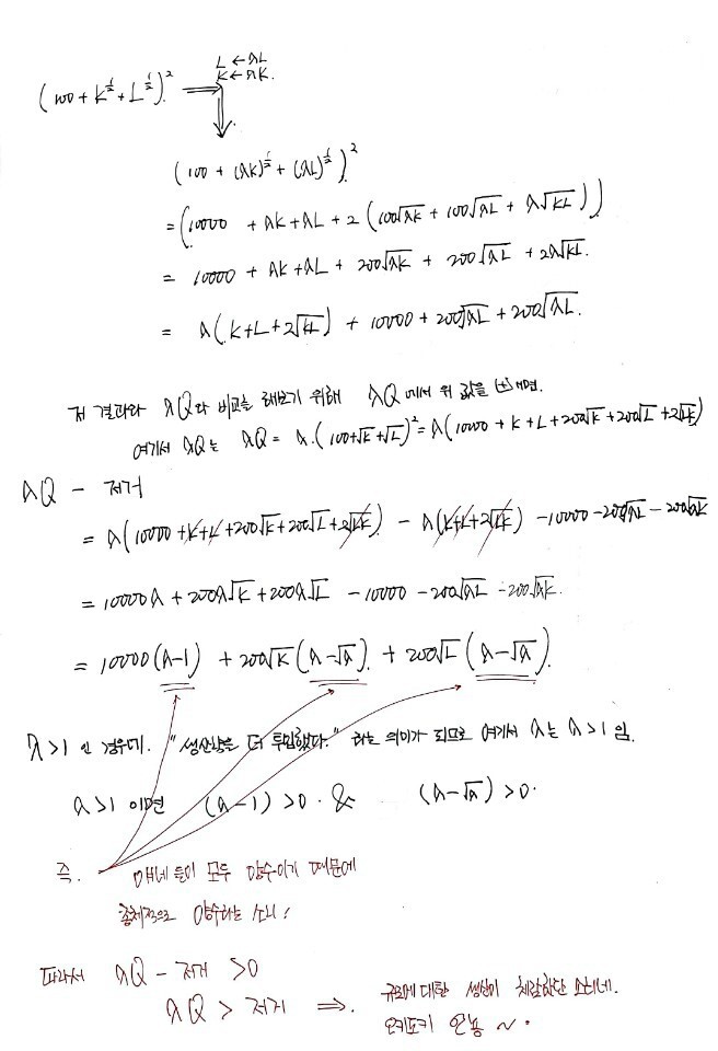
Yoho, constant returns to scale! On to c).

$$Q \quad = \quad \left( \quad 100 \quad + \quad K^{\frac{1}{2}} \quad + \quad L^{\frac{1}{2}} \right)^{2}$$

Plug in $\lambda K$ and $\lambda L$ here!

Prob 6.23

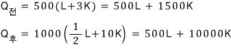
Suppose initially the firm’s production function is

$$Q \quad = \quad 500(L+3K)$$

But thanks to manufacturing-innovation magic, the production function becomes

$$Q \quad = \quad 1000\left( \frac{1}{2}L+10K \right)$$

a) Show that this innovation actually counts as technological progress. b) Is the progress neutral, labor-saving, or capital-saving?

a) is straightforward.

So for the same $(L, K)$ — for any $(L, K)$ whatsoever — we have

$$Q_{\text{before}} \quad < \quad Q_{\text{after}}$$

so yeah, clearly technological innovation went down.

Now to figure out what kind of innovation it is, we need to check the MRTS. The definition is

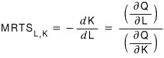
so it works out to

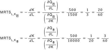
Before, if you cut labor by 60 you had to throw in 20 units of K to keep producing the same Q. Now, if you cut labor by 60, you only need to throw in 3 more units of K to hold Q steady. Which means: in the post-progress era, if it were me, I’d cut a bit of labor and add some K. So we can call this labor-saving technological progress.

---

Originally written in Korean on my Naver blog (2017-01). Translated to English for gdpark.blog.