Introduction to Quantum Mechanics: On Probability [Quantum Mechanics I Studied #1]

Alright — the reason I signed up for the physics department in the first place has finally arrived. Time to study quantum mechanics.

I’m about two weeks into the class as I write this, and… (deep, deep sigh) T_T T_T T_T T_T T_T T_T T_T

Still — maybe the reason this field is extra fun to study is because it’s still very much -ing. Ongoing. Not done.

Mechanics? That belongs to Newton.

Electromagnetism? Maxwell.

Relativity? Einstein.

Each one has a single, undisputed face on the cover.

Quantum mechanics? Apparently… nobody yet. Heh.

Ahhh and let me make this absolutely clear — I am NOT about to become that person, lol. (My foot is already halfway out the door of physics lol lol lol lol — a year in and I’ve felt very keenly this is not water I can swim in.)

Right now, studying quantum just feels like… like I sailed into the Grand Line looking for the One Piece? That’s kind of the vibe when I crack the book open. (Could I be Monkey.G.D.Luffy?? lol)

Ahhh OK that was the vibe at the very beginning of the class. None of that left now. Two weeks in and it’s:

“Oh god I’m so cooked — hair loss red alert!!!” lol that’s all I think about now.

Anyway, enough rambling.

The professor recommended a book to read alongside — I picked up Quantum Story too. Hehehehe hihihi. Let’s go one more round, you and me.

The Schrödinger Equation

In Newtonian mechanics, you solve everything with $F=ma$. That thing is just… truth. Pure truth.

So what’s the equivalent in quantum? The Schrödinger equation. That’s the $F=ma$ of this whole game.

In Newtonian mechanics, you wanted to find $x(t)$.

In quantum mechanics, what you want to find is the wave function $\psi(\mathbf{r},t)$ of a particle.

Just like $F=ma$ gives you $x(t)$, the Schrödinger equation gives you $\psi(\mathbf{r},t)$.

So let me just throw the thing on the page first:

$$i\hbar \frac{\partial \psi}{\partial t} = -\frac{\hbar^{2}}{2m}\nabla^{2}\psi + V\psi = H\psi \\ \begin{cases}\hbar = \dfrac{h}{2\pi} = 1.054{\cdots} \times 10^{-34}\;[\,J \cdot s]\\[6pt]H : \text{Hamiltonian} : E+V = \dfrac{p^{2}}{2m} + V\end{cases}$$

…yeah. Right out of the gate it feels like reading an alien language. T_T

Heh, the Greek letter psi — first time I’m actually writing it. And the Hamiltonian. What is this thing.

(I think this is a quirk of Griffiths, honestly — he plops the result down first and then slowly slots the pieces in one by one by one.)

(But Griffiths is absolutely not a bad book. The practice problems are gems. Practice problems with real meaning, placed exactly where they need to be… God-tier Griffiths.)

(Then again, electromagnetism was the same way for me, so I just shrugged and rolled with it. Heh.)

(By the end of that semester I did get that “ohhh, that’s what I was doing this whole time” feeling lol lol. The easy stuff at the front, you know.)

(So I’ll just keep going.)

Hmm… so what is a wave function?

Apparently the position and the velocity at time $t$ are all wrapped up inside it… uh, what?

For now, the wave function is, mathematically, just a complex number.

So what does it physically mean?

While every genius on Earth was chewing on that question, a guy named Max Born stepped up and said:

(Max Born: hey guys, math genius here — the thing itself doesn’t mean anything! You have to square it for the meaning to fall out!! And the meaning is: the probability density of finding the particle at position $\mathbf{r}$ at time $t$. ~~~~~~~~~)

OK so if we take the genius’s word for it:

$$\int_{a}^{b}{\left|\psi(x,t)\right|^{2}dx} : \text{probability of finding the particle at time } t \text{ between } x=a \text{ and } x=b \\ \Bigl(\left|\psi(x,t)\right|^{2} = \psi^{*}\psi\Bigr) \\ (\psi^{*} \text{ is the complex conjugate of } \psi)$$

(Quick fun aside.) Einstein heard this and absolutely lost it.

“lol lol lol lol lol oh this is utter nonsense lol lol lol
You measured it and it was there, so it was there from the beginning, duh.
What is this nonsense lol — we just didn’t know, and the act of measuring let us see it was there. What do you mean probability. Probability.
Ha………. and these clueless people are physics students…….. are you really physics students after saying things like that??
End of days, end of days~~~~ Add a few more variables we don’t know about yet, predict properly, and you’ll absolutely figure it out, you fools (-_-)
You’re studying an incomplete field and slapping the name ‘quantum mechanics’ on it, you idiots!!!!! you fools!!! >0<”

The other camp — the so-called Copenhagen school — apparently went something like:

“Sir… we hear you, sir… but uh, look at these experimental results over here~”

Einstein: “OK now here’s a thought experiment from the top of my head, listen up, look at this, look at this —”

“Sir… heh, again, here… look at this lol, the experimental data —”

They went at each other absolutely full tilt apparently lol.

Einstein went to his grave never accepting this thing called quantum mechanics. That’s just how it went, apparently. lol lol.

Anyway — the Copenhagen interpretation is the one we treat as (for now) correct, and after John Bell’s experiment everyone basically had to shut up and sit down. Heh.

The crux of the Copenhagen view: it puts the interaction between the act of measurement and the thing being measured at the center.

Because the act of measuring itself changes the thing — you cannot claim the position you measured was the position right before you measured.

OK. So all of the above was the setup for one big idea: this thing called quantum mechanics is deeply tangled up with this thing called probability.

So now we need to circle back and review that probability stuff. Section 3. Probability.

Probability — discrete variables

Say you’ve got a classroom of $N$ students and you want to bin them by age. Age is a discrete number, so let $N(j)$ be the number of students of age $j$.

Then the fact that there are $N$ students total can be written as

$$\sum_{j} N(j) = N$$

Now, common-sense check: if you grab exactly one person, the probability that person is age $j$ is

$$\frac{\text{number of students aged } j}{\text{total number of students}} = \frac{N(j)}{N}$$

Call this $P(j)$ — $P$ for Probability.

$$P(j) : \text{probability that, picking exactly one person, they're age } j$$

Then

$$\sum P(j) = 1$$

is also pure common sense, right? It’s the sum of all the probabilities.

$$\begin{align*} \sum P(j) &= \frac{N(0)}{N} + \cdots + \frac{N(23109)}{N} + \cdots \\ &= \frac{\sum N(j)}{N} \\ &= \frac{N}{N} \\ &= 1 \end{align*}$$

Now we want a single representative number for the class — the average age. How do we get it?

Just think back to how you crunched out your average score in middle school and high school — same deal.

Average. Mean. Expectation value.

$$\text{average of } j = \langle j \rangle = \sum jP(j)$$

OK so to wrap up, this is just the probability and statistics from high school math, very simply.

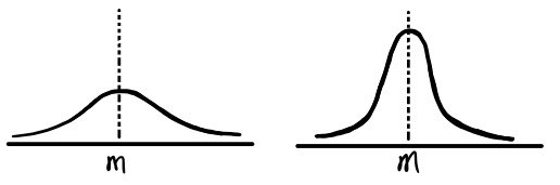
Now look — here are two distributions. The averages of the two data sets are the same, but you can clearly see they’re different, right?

We’re going to learn something that captures that difference.

Call it $\Delta j$ — how far each individual $j$ sits from the mean $\langle j \rangle$.

$$\Delta j = j - \langle j \rangle$$

OK, now let’s average that — the average distance from the average.

Buuuut wait. If you take the average of $\Delta j$,

obviously $\langle \Delta j \rangle = 0$ is going to fall out, right? Because that’s literally what the average means.

So instead — square those distances first, average that, then take the square root!

(Oh man, high school math is coming back to me lol.)

For now,

$$\begin{align*} \langle \Delta j^{2} \rangle &= \sum P(j)(\Delta j)^{2} \\ &= \sum \Bigl((j - \langle j \rangle)^{2}\Bigr)P(j) \\ &= \sum \Bigl((j - \langle j \rangle)^{2}\Bigr)P(j) \\ &= \sum (j^{2} - 2j\langle j \rangle + \langle j \rangle^{2})P(j) \\ &= \sum j^{2}P(j) - 2\langle j \rangle\sum jP(j) + \langle j \rangle^{2}\sum P(j) \\ &= \langle j^{2} \rangle - 2\langle j \rangle\langle j \rangle + \langle j \rangle^{2} \cdot 1 \\ &= \langle j^{2} \rangle - \langle j \rangle^{2} \end{align*}$$

We write this as

$$\sigma^{2}$$

and read it as variance, right?!

And put a square root on it and you get — standard deviation!

$$\sigma = \sqrt{\langle j^{2} \rangle - \langle j \rangle^{2}}$$

Continuous variables

This is what the whole discrete setup was warming us up for.

We used “age” as a discrete variable — fine — but now what about continuous? Hmm.

The book gives a more precise age as the example.

(e.g. my age right now! 24 years 7 months 14 hours 51 minutes 23,..24….25… seconds — (still counting))

Anyway, the probability:

$$P_{ab} = \int_{a}^{b}{\rho \, dx} \\ \begin{cases}\rho : \text{probability density function} \;(\text{probability density})\\[4pt]cf.)\displaystyle\int_{-\infty}^{\infty}{\rho \, dx = 1}\end{cases}$$

This part isn’t unfamiliar — high school did this.

But then — why did we just bother walking through all that obvious stuff with the discrete case?

$$\langle j \rangle = \sum jP(j)$$

This. This is why.

Get the feel for it.

So that, when the variable isn’t chopped into discrete chunks like $j$, you can still find the average without freaking out.

So — for a continuous variable $x$, the expectation value of $x$ is:

$$\langle x \rangle = \int x\rho(x)\,dx$$

Like that! Booom. Beautiful.

Now, the probability density that shows up in nature the most is the Gaussian.

(After Gaussian: exponential. Then Lorentzian. Then on and on and on.)

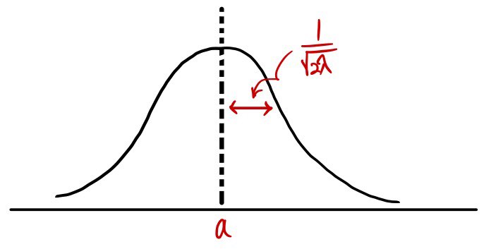
The Gaussian looks like:

$$\rho(x) = Ae^{-\lambda(x-a)^{2}} \quad (x,\,\lambda,\,a > 0)$$

Let’s poke at just one of its features.

$$1.\quad \int_{-\infty}^{\infty}{\rho(x)\,dx = 1}$$

What value of $A$ makes this work?

$$A\int_{-\infty}^{\infty}{e^{-\lambda(x-a)^{2}}}\,dx = 1 \\ \begin{cases}x - a = t\\dx = dt\end{cases} \\ \left(A\int_{-\infty}^{\infty}{e^{-\lambda t^{2}}}\,dt = I \;\text{(call it this)}\right) \\ \begin{align*} I^{2} &= A^{2}\iint e^{-\lambda(x^{2}+y^{2})}\,dx\,dy \;\to\; \text{now switch coordinates} \\ &= A^{2}\int_{0}^{2\pi}\int_{0}^{\infty}e^{-\lambda r}\,r\,dr\,d\theta \\ &= A^{2}\frac{\pi}{\lambda} = 1 \end{align*} \\ \therefore\; A = \sqrt{\frac{\lambda}{\pi}}$$

So with $A = \sqrt{\lambda/\pi}$, the normalization $\int_{-\infty}^{\infty}{\rho(x)\,dx} = 1$ checks out.

$$2.\quad \text{Find } \langle x \rangle.$$$$\begin{align*} \langle x \rangle &= \sqrt{\frac{\lambda}{\pi}}\int_{-\infty}^{\infty}{x\,e^{-\lambda(x-a)^{2}}}\,dx \\ &= a \end{align*}$$$$\begin{align*} 3.\quad \langle x^{2} \rangle &= \sqrt{\frac{\lambda}{\pi}}\int_{-\infty}^{\infty}{x^{2}\,e^{-\lambda(x-a)^{2}}}\,dx \\ &= \frac{1}{2\lambda} + a^{2} \end{align*}$$$$\begin{align*} \therefore\; \sigma^{2} &= \langle x^{2} \rangle - \langle x \rangle^{2} \\ &= \frac{1}{2\lambda} \end{align*} \\ \therefore\; \sigma = \sqrt{\frac{1}{2\lambda}}$$

What it means:

Originally written in Korean on my Naver blog (2015-08). Translated to English for gdpark.blog.