Normalization

That thing I just did….

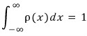
Just like I fixed the value of the constant A that makes this… happen,

hmm~~~ ah so

becomes the probability density function! After finding that out!!!

since we know that this functions as the probability density function, next, so that its function works properly

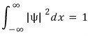
so that this holds!!! I think it’s better to think of it as scaling by a constant!

That whole process of scaling it to 1 with a constant like that is called Normalization/

<The book says it too!!! “Without this condition, the statistical interpretation is meaningless.”>

Okay so now we kinda know what normalization is~~

But during class the professor said this, and the book also says that thinking about this process is important

what exactly do we think about~~

Alright let’s see. The ψ function is a function of position x and time t, ya know, but say we did the normalization at t=0.

eh~~ but after a little time passes, do we have to normalize again?

this this this this

And the answer to this is That’s a nope nope nopety-nope

Why?????????????????

That secret !!! lies in the Schrödinger equation.

Just as in classical mechanics all secrets are held by F=ma,

in quantum mechanics the secret is contained in the Schrödinger equation!!!!

Let’s say this has been normalized! Then

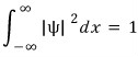
this is satisfied

and now the Question is

as time goes on, does it conti~~~~~~~~~~~~nue to

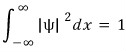
satisfy this, that’s what we’re asking

so we

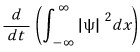
just have to compute this once.

And, if that calculation result is 0 then we can answer Yes

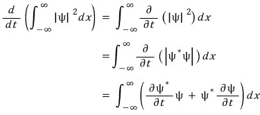
Start!

Source correction — 2026-10-01: The preceding image preserves the equation printed in my 2015 post. Its kinetic term has a typo: the second derivative should be with respect to position, as in the next two images. For a particle of mass $m$ in one dimension, the equation used here is

$$ i\hbar\frac{\partial\psi}{\partial t} =-\frac{\hbar^2}{2m}\frac{\partial^2\psi}{\partial x^2}+V(x,t)\psi. $$

using this

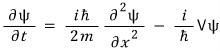
and automatically

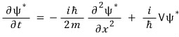
we substitute this in here!!

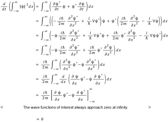
Boundary note — 2026-10-01: The preceding image preserves my original statement about wave functions approaching zero at infinity. This calculation assumes a square-integrable state, a real potential, and sufficient regularity for the derivatives and boundary limits. Writing $N(t)=\int_{-\infty}^{\infty}|\psi|^2\,dx$ and $j=(\hbar/m)\operatorname{Im}(\psi^*\partial_x\psi)$ gives

$$ \frac{dN}{dt}=-\bigl[j(+\infty,t)-j(-\infty,t)\bigr]. $$

Vanishing current at both infinities is sufficient. For example, $\psi\to0$ together with bounded $\partial_x\psi$ makes each current vanish; $\psi\to0$ alone does not control the derivative. An ideal plane wave on the full line is not square-integrable and cannot be normalized to one by a finite constant.

Anytime, anywhere, if it gets normalized once

then even after time flows, it maintains the normalized state~~~~~~ I think we can understand it that way.

Scope note — 2026-10-01: My original “Anytime, anywhere” conclusion refers to the total norm of the full state under unitary Schrödinger evolution. A time-independent self-adjoint Hamiltonian generates such evolution; a time-dependent Hamiltonian also requires a well-defined unitary evolution. In the real-potential calculation above, the operator’s domain and boundary conditions must justify the boundary step. Probability within a smaller spatial interval can change as current crosses its ends. Non-unitary effective evolution can also change a state’s norm, so the conclusion is not unconditional.

Original post: Normalization (2015)