The Momentum Operator

I’ll continue right where I left off.

When a particle’s wavefunction (state function) is ψ(x,t), the probability??? (expectation value) of the particle being at position x is!!

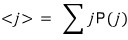
In the same vein,

for the continuous variable x,

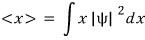
we can say.

What the professor told us in class so we wouldn’t get confused about the meaning of this <x> was

that the probability of being at position x does NOT mean

that if you measure this ψ particle continuously! repeatedly, you’ll arrive at <x>,

but rather, it’s the average!!! of the results when many people measure this ψ,

and this is what the perfessor, and the book, both emphasize (I think he was emphasizing the point of it being an ensemble average).

Editorial clarification (1 October 2026). The opening formulas give the expectation value of position, not a probability. For a normalized wavefunction, $\rho(x,t)=|\psi(x,t)|^2$ is a probability density, $P(a\le x\le b)=\int_a^b|\psi(x,t)|^2\,dx$, and $\langle x\rangle=\int_{-\infty}^{\infty}x|\psi(x,t)|^2\,dx$. The average concerns identically prepared systems measured at the same evolution time t: separate copies, or the same system prepared again before each trial. Several people are not required. Repeatedly measuring one system without preparing it again generally samples a changed state. See MIT Lecture 8, §2 and MIT Chapter 2, §2.3.4.

Alright, so now I kind of get the meaning of <x>.

Then as t changes in the state function, the probability of the particle being at x at that time also changes, right???

Following the trend of change of the expectation value of position as time changes — let’s call this the velocity of the x expectation value! <v>?

Anyway, what I’m trying to do is differentiate <x> with respect to t!!!

It’s very similar to the integration method we did before!!

Starting!!!!!! (You’ll gradually come to see what this is all about, so let’s just calculate first.)

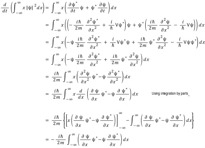
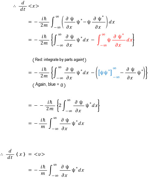
Editorial correction (1 October 2026). The source image above has two intermediate typographical errors: a missing integral in the integration-by-parts line and an extra minus in the next line. Its final sign is correct. For the one-dimensional Hamiltonian $\hat H=-\hbar^2\partial_x^2/(2m)+V(x,t)$, take real $V$, constant positive $m$, and a normalized, sufficiently smooth state with finite expectations and enough decay for the integrals, time differentiation and boundary limits below. Normalization alone does not justify discarding boundary terms. With $\psi'=\partial_x\psi$, the corrected steps are:

$$ \int_{-\infty}^{\infty}\psi(\psi^*)'\,dx=[\psi\psi^*]_{-\infty}^{\infty}-\int_{-\infty}^{\infty}\psi'\psi^*\,dx, $$$$ \frac{d\langle x\rangle}{dt}=-\frac{i\hbar}{2m}\left(2\int_{-\infty}^{\infty}\psi'\psi^*\,dx-[\psi\psi^*]_{-\infty}^{\infty}\right)=-\frac{i\hbar}{m}\int_{-\infty}^{\infty}\psi^*\psi'\,dx. $$

The last equality uses $[\psi\psi^*]_{-\infty}^{\infty}=0$; the preceding image also uses $[x(\psi'\psi^*-\psi(\psi^*)')]_{-\infty}^{\infty}=0$. These are full-real-line integrals. Other spatial domains require their own boundary conditions. This derivation is obtained by substituting the Schrödinger equation and integrating by parts; the MIT operator formalism supplies the Hamiltonian and expectation conventions.

If this is the expectation value of the particle’s velocity, (or should I say ’the velocity of the particle’s position expectation value’?)

let me multiply by m to get the expectation value of the momentum.

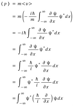
Editorial correction (1 October 2026). One intermediate line in the source image drops the factor $-i\hbar$. It must remain until it is written as $\hbar/i$. Under the assumptions just stated, the full-real-line identity is

$$ \langle p\rangle=m\frac{d\langle x\rangle}{dt}=-i\hbar\int_{-\infty}^{\infty}\psi^*\partial_x\psi\,dx=\int_{-\infty}^{\infty}\psi^*\left(\frac{\hbar}{i}\partial_x\right)\psi\,dx. $$

Thus $\hat p=-i\hbar\partial_x$. The derivative acts on the wavefunction to its right; the integral produces the expectation value. See MIT Lecture 8, §2.

Alright alright alright, let me pull out just two of those integrations we were doing like crazy earlier and write them down again.

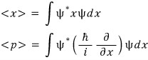
The book says

‘x’ is not just ’the position x’, but “represents x~~”

‘p’ is not “just the momentum p”, but “represents p~~~”

that’s what it means,

but I want to re-express this in my own way so it really hits home.

Looking at the result, p is

this thing,

and some “momentum value!!!” — the important thing is, in quantum mechanics, p the momentum is not a ‘value’,

but something you apply to get the expectation value <p>!!! (from now on, p is not a value but an ‘operator’)

This is how I understood it,

and if you understand it in this context​

(from here on it’s nonsense)

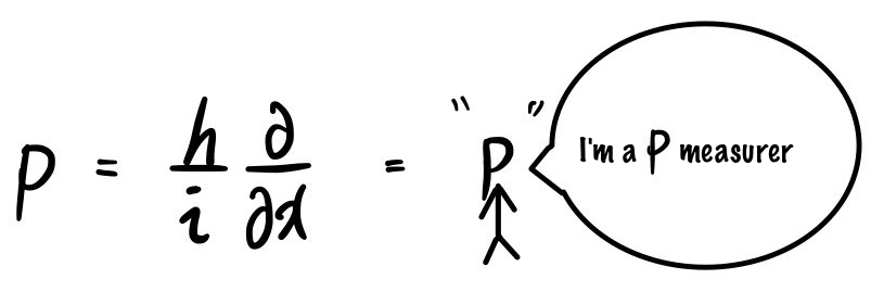
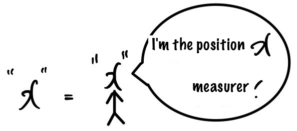
These are the kind of guys it’s talking about, I think…

When you’re curious about a particle’s p,,,,

now

you go talk to this guy.

Me: “Hey you, p-measurer! Measure p for me!”

“Yeah got it, bring the particle state function and I’ll measure it for you!!”

Me: “Yup~~~ here

this one~~~ and

this is the complex conjugate!!!!”

Yeah!!! Stick those two on either side of me and smash an integral on it!!!!

Then I’ll disappear T_TT_T Once I disappear, look at what comes out! Gotchu?!!!

byeeee…..

(What I wanted to say is that p is an operator, but I don’t know if it’s okay to talk like I’m on drugs like this T_TT_TT_T)

While just spouting nonsense, what hit me was that talking this kind of crazy talk actually gave me a bit of insight into why the Copenhagen school

emphasized the interaction between the experimental subject and the experimenter….heh.heh.

Editorial clarification (1 October 2026). The ‘measurer’ cartoon is the author’s mnemonic. Applying $\hat p$ to $\psi$ produces a function, generally unnormalized; forming $\int\psi^*\hat p\psi\,dx$ produces the expectation value, not generally the result of a single measurement. An individual ideal measurement returns an outcome from the observable’s spectrum. The Copenhagen remark records the author’s personal association and is not a historical derivation of that interpretation. See MIT Chapter 2, §§2.2–2.3.

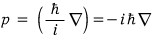
cf.) I wrote p in one dimension as

but if we expand it to 3 dimensions ~

okaaay????

One more thing — the ’energy!’ that I originally understood as a ‘value’,,,

after we’ve changed our concept of momentum,,,,

let’s see what transformation energy’s shape undergoes in quantum mechanics​

so~

Then the expectation value for T is…heh

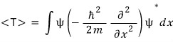
Editorial clarification (1 October 2026). The standard expectation formula places $\psi^*$ on the left and lets the operator act on $\psi$ to the right:

$$ \langle T\rangle=\int_{-\infty}^{\infty}\psi^*\left(-\frac{\hbar^2}{2m}\partial_x^2\right)\psi\,dx. $$

The source image reverses these two functions. For this real-coefficient kinetic operator, the reversed integral is the complex conjugate of the standard one. On a suitable self-adjoint domain the expectation is real, so both give the same value; this does not justify reversing them for a general operator. With sufficient regularity and $[\psi^*\partial_x\psi]_{-\infty}^{\infty}=0$, integration by parts also gives $\langle T\rangle=\frac{\hbar^2}{2m}\int_{-\infty}^{\infty}|\partial_x\psi|^2\,dx\ge0$. Normalization alone is insufficient for these boundary and domain requirements. See MIT Chapter 2, §§2.2 and 2.3.4.

Why do I keep placing it in the middle between the wavefunction and its complex conjugate when computing expectation values — the reason for this, honestly, you learn in chapter 3…..

Well…. until then I was just like ohhh okay~~ and kind of went with it,

but you can just think of it as ’that’s the definition’!

P.S.

This was a post where I was emphasizing the ‘measurer’ aspect of the operator.

What can we call this act of measuring, mathematically?

Couldn’t we call it a ‘matrix’??

That is, momentum is a matrix…. which in turn means…

the act of differentiation itself becomes describable as a matrix.

‘differentiation is a matrix’

I recently enjoyed a YouTube video that introduces this,

and I think it will help understand this post veryveryveryveryvery much,

so even though it’s way later than when this post was actually written, right now,

I’m putting up this link…..

(goosebumps. goosebumps….)

https://youtu.be/BaEillNU3Nk

video

The simulation universe discovered in quantum mechanics

【Related videos and blog postings】— Differentiation is a matrix (https://youtu.be/RZkTxmUWcns)— Differentiation is a matrix (https://moe34.tistory.com/18)— Mi…

The source card excerpt ends with an incomplete Korean word, transliterated here as “Mi…”. The missing text is not reconstructed.

youtu.be

Editorial clarification (1 October 2026). Differentiation is a linear operator. Once an orthonormal basis is chosen, its action has a matrix representation, with entries $D_{mn}=\langle e_m|\partial_x e_n\rangle$ when those basis functions belong to its domain. The continuum operator generally requires an infinite-dimensional description; a finite matrix may describe an invariant subspace exactly or a chosen approximation. The basis and operator domain, including boundary conditions, matter. See MIT Chapter 2, §2.2.

Original Korean notes (11 August 2015)