The Finite Square Well
Tackling the finite square well — the sneaky middle ground between the infinite well and the delta function — through bound states, boundary conditions, and all that fun stuff.
Man… there are just so many potentials. HELL HELL HELL HELL!!!! Why are there this many of them, and why are they all this hard?? lol
But OK — this really is the last one!!! Muster up, let’s go!!!
Here’s the shape:
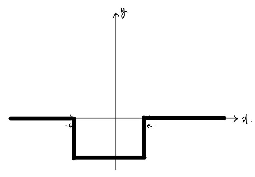
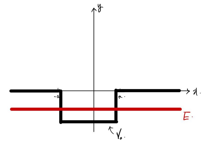
$V_0$ is a constant, a real number greater than 0. Constant!
This isn’t an infinite square well, and it isn’t a δ-function either…
Something kinda sitting in between those two~~~~
Anyway.
Same as always, there’s going to be both a bound state and a scattering state.
And same as always, let’s look at one case of each.
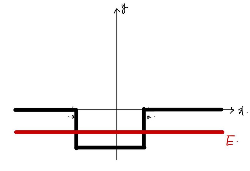
Bound state first!!!!
For the bound state $E < 0$, so it looks like this~~~~~
Starting from
$$-\frac{\hbar^2}{2m}\frac{d^2\psi}{dx^2} + V(x)\psi = E\psi$$let’s hit the region $x < -a$ with the time-independent Schrödinger equation, step by step!!!~~~
$$\frac{d^2\psi}{dx^2} = -\frac{2mE}{\hbar^2}\psi = K^2\psi \quad \left(K = \frac{\sqrt{-2mE}}{\hbar}\right)$$Just like we did with the delta-function potential well — since $E$ is negative, that whole red chunk including the minus flips positive~~!~!!
Hella familiar.
General solution for $\psi(x)$ in $x < -a$:
$$\psi(x) = Ae^{Kx} + Be^{-Kx}$$but~~~ to stop it blowing up at $x = -\infty$, $B = 0$ !!!!
OK so — general solution for $\psi(x)$ when $x > a$ is
$$\psi(x) = Fe^{Kx} + Ge^{-Kx}$$and to stop it blowing up at $x = \infty$, $F = 0$ !!! Right?!
(Wait — back at the delta well I called this one $G$. Different letter now. Sorry, notation drift.)
OK so what happens in $-a < x < a$?….. (a little tense;; T_T)
$$-\frac{\hbar^2}{2m}\frac{d^2\psi}{dx^2} - V_0\psi = E\psi$$Schrödinger becomes:
$$\frac{d^2\psi}{dx^2} = -\left\{\frac{2m}{\hbar^2}(E + V_0)\right\}\psi = -l^2\psi \quad \left(l^2 = \frac{2m(E+V_0)}{\hbar^2}\right)$$<This one can trip you up, but the red bit is positive. Because $V_0$ is positive. Right?!? $V_0$ is positive!!! heh heh heh>
$E$ is negative!!!
And in magnitude, $V_0$ is the bigger one.
OK?
Shall we write the general solution for $\psi(x)$ in $-a < x < a$ as
$$\psi(x) = Ce^{lx} + De^{-lx}$$??
We could. It’s not wrong. But for the algebra later it’s way cleaner to write it as
$$\psi(x) = C\sin lx + D\cos lx$$(Remember when we cracked the Laplace equation back in the electromagnetism potential post? Same deal.)
Stacking up everything we’ve got so far:
$$\psi(x) = \begin{cases} Fe^{-Kx} & (x > a) \\ C\sin lx + D\cos lx & (-a < x < a) \\ Ae^{Kx} & (x < -a) \end{cases}$$Now — time to match boundaries. Condition: $\psi(x)$ is continuous.
And — remember the other condition we used last time?
(Dirac potential well!) Back there we integrated from $-0$ to $+0$!!!
But that was basically equivalent to saying “$\psi'(x)$ is continuous”!!!
Same trick works here — if we integrate from $a-0$ to $a+0$,
$$\Delta\left(\frac{d\psi}{dx}\right) = 0$$pops out.
So since we already know this~~~~~~ let’s just use “$\psi'(x)$ is continuous” directly.
(At $x = a$, $\psi(x)$ continuous →)
$$Fe^{-Ka} = C\sin la + D\cos la$$(At $x = a$, $\psi'(x)$ continuous →)
$$-KFe^{-Ka} = Cl\cos la - lD\sin la$$(At $x = -a$, $\psi(x)$ continuous →)
$$Ae^{-Ka} = C\sin l(-a) + D\cos l(-a) \\ = -C\sin la + D\cos la$$(At $x = -a$, $\psi'(x)$ continuous →)
$$KAe^{-Ka} = Cl\cos l(-a) - Dl\sin l(-a) \\ = Cl\sin la + Dl\cos la$$Now — $V(x)$ is symmetric about the y-axis. It’s an even function.
Which means $\psi(x)$ has to be either even or odd — same story as the infinite square well!!
$\psi(x)$ must be one of the two. No other option.
So let’s split into cases — even, and odd.
Even case first!!!!
$$\psi(x)_{\text{even}} = \begin{cases} Fe^{-Kx} & (x > a) \\ D\cos lx & (-a < x < a) \\ Fe^{Kx} & (x < -a) \end{cases}$$We apply the boundary conditions — but since it’s even, we don’t need to check both $x = a$ and $x = -a$. Just $x = a$ is enough.
$$\text{B.C.} \\ \psi(x) \text{ continuous} \to Fe^{-Ka} = D\cos la \\ \frac{d\psi(x)}{dx} \text{ continuous} \to -KFe^{-Ka} = -lD\sin la$$$$\text{Divide one by the other:} \\ l\tan(la) = K$$Boom, there’s our relation.
Now to actually find the solution… we should remember what $l$ and $K$ are in the first place~~~~~:
$$K = \frac{\sqrt{-2mE}}{\hbar}, \quad l = \frac{\sqrt{2m(E+V_0)}}{\hbar}$$So~~~~~~ both $l$ and $K$ are functions of the energy $E$. And, using both of them, we can cook up one more relation:
$$K^2 + l^2 = \frac{2mV_0}{\hbar^2}$$(Honestly I should’ve written this relation way~~~ up there and dragged the equation down here, but it suddenly looks out of place now… T_T ugh…)
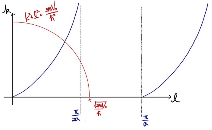
$$\begin{cases} l\tan(la) = K \\ K^2 + l^2 = \dfrac{2mV_0}{\hbar^2} \end{cases}$$So we need $l$ and $K$ satisfying both of these….
Hmm — can’t we just draw an $l$-axis and a $K$-axis and look for intersection points?????
Because an ordered pair $(l, K)$ sitting on both curves is exactly an $l$ (and matching $K$) that satisfies the top equation AND the bottom equation~~!
OK! Here we go:
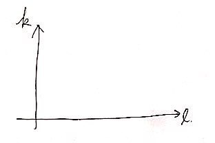
Plot both curves on those axes, hunt for intersections.
And hold onto this: the $K$ and $l$ we find represent Energy.
Which means — an intersection existing is the same as saying there’s an $E$ that satisfies both equations. Which is the same as saying a bound state exists!!!! haha
I guess that’s the whole point of drawing graphs and hunting intersections~~~~~~ heh
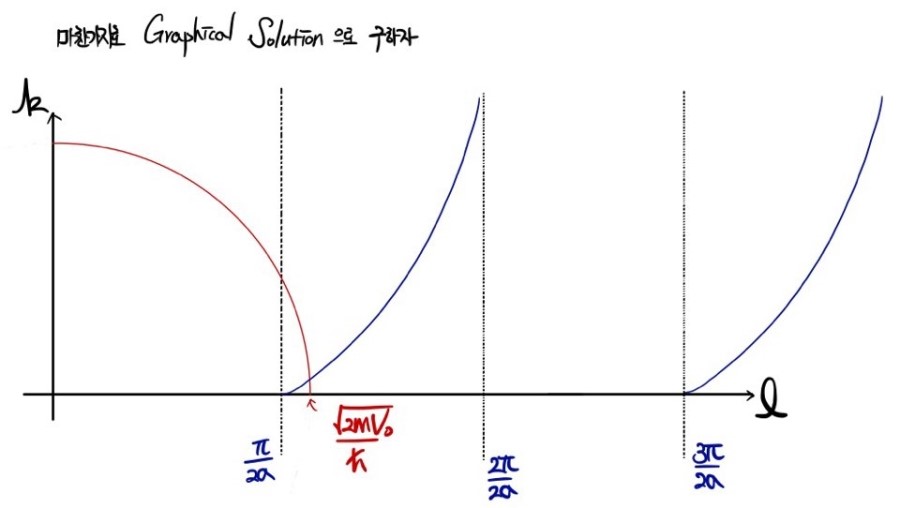
So let’s pull the Solution off those intersection points. (Apparently this kind of move is called a Graphical Solution.)
$K$ and $l$ are both positive!!!! so we don’t need the whole plane — first quadrant only.
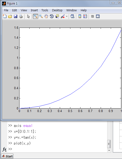
Just to be safe, I plotted $x\tan x$ in Matlab!!
And combined both curves on paper.!!!!
Now what we actually want to check is: does an $E$ exist at all?
That is — no matter what the setup is, does at least one intersection always exist?
That there’s always at least one — you’d spot it immediately with your own eyes.
And how many solutions exist~~~ (how many possible $E$’s, how many possible bound states~~~) would be the thing to actually nail down.
But… nah, let’s skip that. T_T
Let’s just check the two limiting cases. The extreme setups!!!
That alone will answer the question above.
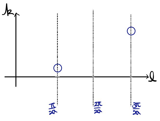
* Case 1: super~~~~~~~ wide and super~~~~~~~ deep well!!!!!!
$a$ is huge, so $1/a$ is ridiculously tiny.
I can’t say for sure, but — if a solution exists, that solution is almost~~~~ right on the asymptote!!!! (because $a$ is huge.)
That is, the solutions for $l$ are
$$l \cong \frac{\pi}{2a}n$$we can say~~~~ ($n$: odd!)
** Case 2: the other limit!!
Ridiculously narrow and also ridiculously shallow well!!!!!
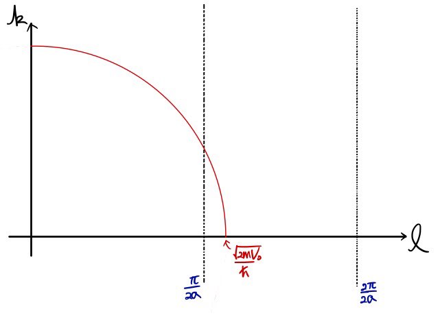
In this regime, $V_0$ is so small that a situation can arise where only one solution exists!!
Because $a$ is ridiculously~~~~~~~~~~~~~~~ small, the asymptote sits oh~~~~~~~~~~ so far away.
BUT!!! No matter how far the asymptote is, no matter how far, you can absolutely!!!!!!!!!!!! always get at least one solution, no exceptions.
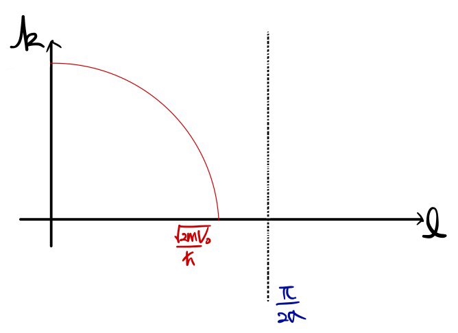
So how small does $V_0$ have to be before you’re down to a single solution? When it looks like the picture above — exactly one solution:
$$\frac{\sqrt{2mV_0}}{\hbar} < \frac{\pi}{2a}$$One in that case.
Honestly though, the real point isn’t how many solutions there are. It’s that for the finite square well, there’s no such thing as “no state is possible”!!!!! Something always exists.
※Warning: heart attack risk※
Everything so far was only for $\psi(x)$ even.
Half is still left……
When $\psi(x)$ is odd — those cases exist too. Let’s hit them.
Odd case
$$\psi(x)_{\text{odd}} = \begin{cases} Fe^{-Kx} \\ C\sin lx \\ -Fe^{-Kx} \end{cases}$$Apply the B.C.s the same way:
$$Fe^{-Ka} = C\sin la \\ -KFe^{-Ka} = lC\cos la$$Two equations, giving the relations
$$K = -l\cot(la) \\ K^2 + l^2 = \frac{2mV_0}{\hbar^2}$$OK~~~
Oh~~~~~
If $V_0$ is too small compared to $1/a$, there might be no solution????
Same move as before — limiting cases!!!!!
1.) Super wide and super deep well.
Again — if $a$ is huge, $1/a$ is tiny~ so there’ll be lots of solutions~~~
Same idea, I can’t say for sure, but the intersections sit near the next asymptote over (this is the difference!!!)
$$l \cong \frac{\pi}{2a}n$$($n$ even)
Substituting into
$$l = \frac{\sqrt{2m(E+V_0)}}{\hbar}$$$$\therefore \quad E_n + V_0 = \frac{\hbar^2}{2m}\left(\frac{\pi n}{2a}\right)^2$$‘In this regime a solution definitely exists!!!’
- Super narrow, super shallow well.
Same deal — we pin it down by the “radius” like before.
But this time, if $a$ gets too small and $1/a$ gets big, and that gap gets too too large, we might end up with no solution at all.
So — let’s also find the case with exactly~~~!!! one solution.
Outside that range: zero solutions, or else 2+ solutions! Either way!!
Exactly~~~ one solution happens when
$$\frac{\pi}{2a} < \frac{\sqrt{2mV_0}}{\hbar} < \frac{2\pi}{2a}$$exactly this range~~~~~~~~~~~~~ *>0<*
P.S. The reason I kept banging on about “one case, one case” this whole time —
it’s because there’s a regime where only one wavefunction state is possible!! heh
OK I really should switch departments.
What was the department office phone number again…. >3
Originally written in Korean on my Naver blog (2015-08). Translated to English for gdpark.blog.