Larmor Precession and the Stern-Gerlach Experiment

This post develops two closely related examples from Griffiths: Larmor precession and the Stern-Gerlach experiment. Together they show how a spin magnetic moment behaves in a uniform magnetic field and how a field gradient turns spin into a measurable spatial separation.

1. Larmor precession

The following sketch is a useful picture of precession, but it should not be read as an electron literally spinning like a tiny rigid sphere. Spin is an intrinsic quantum degree of freedom.

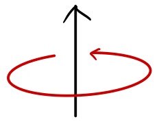
For a particle with spin angular momentum \(\mathbf S\), its magnetic moment is proportional to \(\mathbf S\):

\[ \boldsymbol\mu=\gamma\mathbf S. \]

The proportionality constant \(\gamma\) is the gyromagnetic ratio: it relates magnetic moment to spin angular momentum, not to a classical fast or slow rotation.

For an electron,

\[ \gamma=-g\frac{e}{2m_e}\approx-\frac{e}{m_e}, \]

because the electron spin \(g\)-factor is close to 2. The minus sign matters: the electron’s magnetic moment points opposite to its spin angular momentum. The proton’s magnetic moment is much smaller on this scale, although it is not literally zero.

A magnetic moment in a magnetic field experiences the torque

\[ \boldsymbol\tau=\boldsymbol\mu\times\mathbf B, \]

while its magnetic interaction energy is

\[ U=-\boldsymbol\mu\cdot\mathbf B. \]

If the field varies with position, that energy produces the translational force

\[ \mathbf F=-\boldsymbol\nabla U =\boldsymbol\nabla(\boldsymbol\mu\cdot\mathbf B). \]

An ideal uniform field therefore produces torque and precession but no translational Stern-Gerlach force.

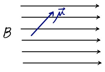
Now apply a uniform external field in the \(z\)-direction:

\[ \mathbf B=B_0\hat{\mathbf z}. \]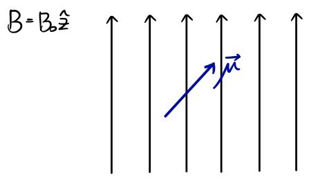

The spin Hamiltonian is

\[ H=-\boldsymbol\mu\cdot\mathbf B =-\gamma B_0S_z. \]

In the \(S_z\) basis,

\[ S_z=\frac{\hbar}{2} \begin{pmatrix} 1&0\\ 0&-1 \end{pmatrix}, \qquad H=-\gamma B_0\frac{\hbar}{2} \begin{pmatrix} 1&0\\ 0&-1 \end{pmatrix}. \]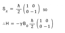

Therefore the basis spinors \(\chi_+\) and \(\chi_-\) are also energy eigenstates:

\[ E_+=-\gamma B_0\frac{\hbar}{2}, \qquad E_-=+\gamma B_0\frac{\hbar}{2}. \]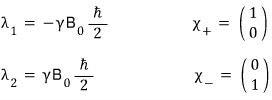

The time-dependent Schrödinger equation is

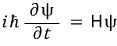
The same equation can be written directly for an abstract state:

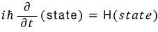
In this basis the two stationary spinors are

\[ |\chi_+\rangle= \begin{pmatrix}1\\0\end{pmatrix}, \qquad |\chi_-\rangle= \begin{pmatrix}0\\1\end{pmatrix}. \]

The original notes display their labels separately:

An energy eigenstate acquires the phase factor

under time evolution.

To see precession, consider the expectation value of the spin vector. The original notes write the spatial integral form

which assumes that any spatial part of the state is normalized. For the two-component spinor used below, the same expectation value is simply \(\chi^\dagger S_x\chi\).

Take an initial state with no relative phase,

and choose the real normalized coefficients

\[ a=\cos\frac{\alpha}{2}, \qquad b=\sin\frac{\alpha}{2}. \]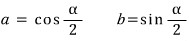

After time \(t\), each energy component carries its own phase:

\[ |\chi(t)\rangle =a e^{-iE_+t/\hbar}|\chi_+\rangle +b e^{-iE_-t/\hbar}|\chi_-\rangle. \]

The expectation value has the well-formed bra-ket and matrix representations

\[ \begin{aligned} \langle\chi(t)|S_x|\chi(t)\rangle &=\chi^\dagger(t)S_x\chi(t)\\ &=\frac{\hbar}{2} \begin{pmatrix} a e^{iE_+t/\hbar} & b e^{iE_-t/\hbar} \end{pmatrix} \begin{pmatrix} 0&1\\ 1&0 \end{pmatrix} \begin{pmatrix} a e^{-iE_+t/\hbar}\\ b e^{-iE_-t/\hbar} \end{pmatrix}. \end{aligned} \]

Here the two energy eigenvalues are

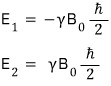
and substituting them gives the relative phase responsible for precession.

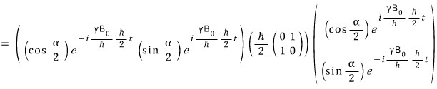
The expectation values are

\[ \langle S_x\rangle=\frac{\hbar}{2}\sin\alpha\cos(\gamma B_0t), \]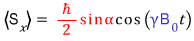

\[ \langle S_y\rangle=-\frac{\hbar}{2}\sin\alpha\sin(\gamma B_0t), \]

and

\[ \langle S_z\rangle=\frac{\hbar}{2}\cos\alpha. \]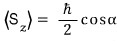

Thus \(\langle\mathbf S\rangle\) keeps a fixed polar angle and rotates about the field axis.

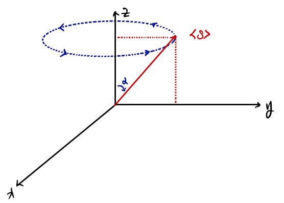
With the convention used here, the signed angular frequency is

\[ \omega_L=\gamma B_0. \]

The observable precession rate is its magnitude, \(|\omega_L|=|\gamma|B_0\); the sign specifies the direction of rotation. This is the Larmor frequency.

2. The Stern-Gerlach experiment

Larmor precession describes spin dynamics in a uniform field. The Stern-Gerlach experiment uses a nonuniform magnetic field so that different spin components experience different forces.

One historical correction is important. Walther Gerlach did not receive a Nobel Prize and was not executed after World War II. He participated in Germany’s wartime uranium project, was detained and interned at Farm Hall in 1945, later returned to academic life, and died in 1979.

The original 1922 experiment used a beam of neutral silver atoms. This was not because atomic hydrogen would cause anything resembling a hydrogen-bomb hazard. Silver was experimentally convenient, and its ground-state electronic configuration is

The closed shells contribute no net electronic angular momentum, while the outer \(5s\) electron has \(l=0\). Neglecting smaller corrections, the atom’s relevant electronic angular momentum is therefore \(J=1/2\), dominated by that electron’s spin. This makes silver a clean two-state example.

Stern and Gerlach sent a collimated beam of silver atoms through specially shaped magnet poles that produced a strong field gradient.

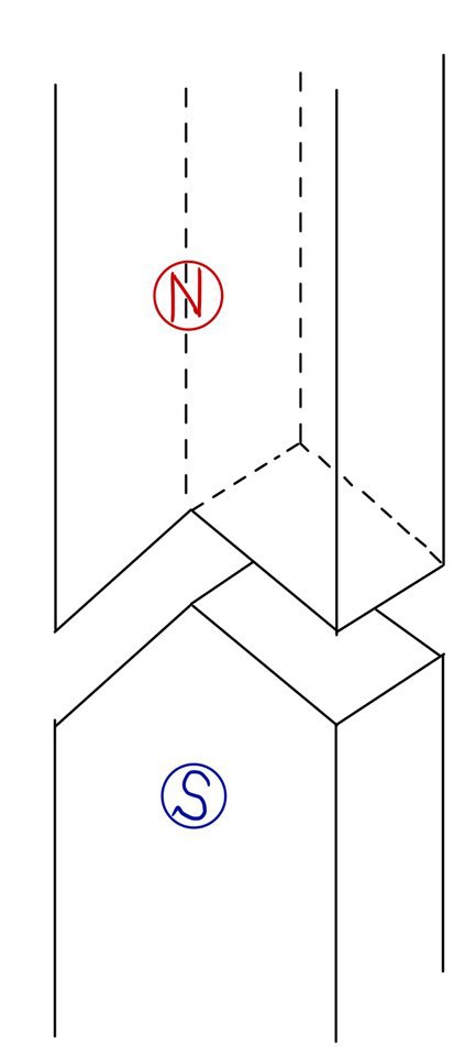
Instead of forming one continuous smear, the beam split into two components.

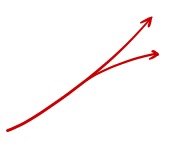
The magnetic interaction Hamiltonian, equivalently the position-dependent potential energy, is

\[ H=U=-\boldsymbol\mu\cdot\mathbf B. \]

Its gradient gives the force:

\[ \mathbf F=-\boldsymbol\nabla U =\boldsymbol\nabla(\boldsymbol\mu\cdot\mathbf B). \]

For orientation, begin with an idealized pair of ordinary, symmetric pole faces.

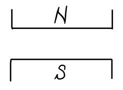
Near the center one might first imagine an approximately uniform field,

but the shaped pole faces make the field vary with position.

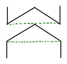
A simple local model is

\[ \mathbf B=(-\alpha x,0,B_0+\alpha z). \]

The intermediate image below displays only the \(z\)-dependent part.

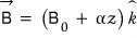
The additional \(-\alpha x\hat{\mathbf x}\) term is required because Maxwell’s equation is

\[ \boldsymbol\nabla\cdot\mathbf B=0, \]

not \(\boldsymbol\nabla\mathbf B=0\). Indeed,

\[ \frac{\partial B_x}{\partial x}+\frac{\partial B_z}{\partial z} =-\alpha+\alpha=0. \]

Using \(\boldsymbol\mu=\gamma\mathbf S\),

the dot product and its gradient are

\[ \begin{aligned} \boldsymbol\mu\cdot\mathbf B &=\mu_x(-\alpha x)+\mu_y(0)+\mu_z(B_0+\alpha z)\\ &=-\alpha\mu_x x+\mu_zB_0+\alpha\mu_z z, \end{aligned} \]

and therefore

\[ \begin{aligned} \mathbf F &=\boldsymbol\nabla(\boldsymbol\mu\cdot\mathbf B)\\ &=-\alpha\mu_x\hat{\mathbf x}+\alpha\mu_z\hat{\mathbf z}\\ &=-\alpha\gamma S_x\hat{\mathbf x} +\alpha\gamma S_z\hat{\mathbf z}. \end{aligned} \]

The minus sign in \(-\alpha\mu_x x\) is retained at every step.

Rapid precession makes the transverse contribution average to zero in the idealized beam treatment, leaving the vertical force

\[ F_z\approx\alpha\gamma S_z. \]

For spin one-half, a measurement of \(S_z\) has only the two eigenvalues \(\pm\hbar/2\). Therefore

\[ F_z=\pm\frac{\alpha\gamma\hbar}{2}. \]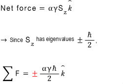

Because \(\gamma\) is negative for an electron, the sign convention determines which spin label bends upward; the essential result is the pair of discrete deflections. In a fuller quantum description, the inhomogeneous field correlates the atom’s spin state with its path, and the detector records one of the two spatially separated outcomes.

That is the central significance of the Stern-Gerlach experiment: angular-momentum components are quantized. The apparatus does not sort pre-existing little classical arrows pointing at arbitrary angles into a continuum. It produces the two outcomes allowed for a spin-1/2 system along the chosen measurement axis.

Modern spin preparation and detection use many techniques, including magnetic resonance, optical methods, spin-polarized transport, and semiconductor devices. The basic lesson of Stern-Gerlach remains the same: a quantum spin component has discrete measurement outcomes.