Two-Particle Systems and the Exchange Force

At last—we have reached Chapter 5.

Until now, we have focused almost entirely on the hydrogen atom. (And that alone took forever.)

Now that we know how to approach hydrogen, let us move on to something new.

It is time to study helium, whose nucleus contains two protons.

A neutral helium atom, of course, also has two electrons.

(To be perfectly clear, we have not even solved hydrogen in every possible sense yet. Ha!)

(As we will discover, helium is not exactly solvable in the same elegant way. It is certainly beyond what an undergraduate course can handle without approximation.)

Before we tackle a two-particle atom, however, we need some new ideas that were unnecessary for a one-particle system.

That is the subject of Chapter 5: identical particles.

Once a system contains two or more electrons, what new issue must we consider?

This one.

Let me illustrate it with a picture.

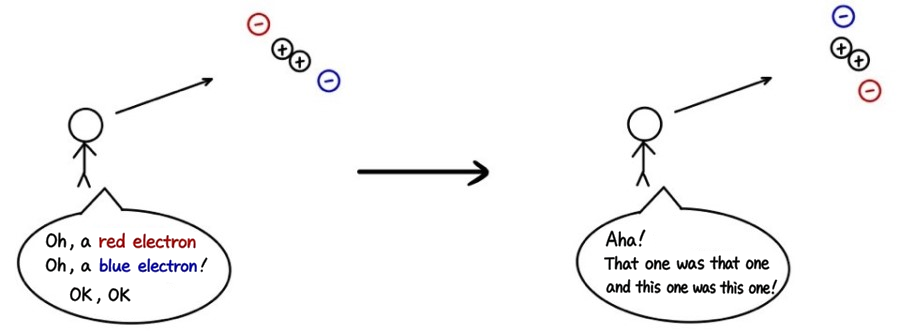
The distinction shown here may seem obvious, but quantum mechanics does not allow us to make it for identical particles.

In other words,

the stick figure in the picture would say this:

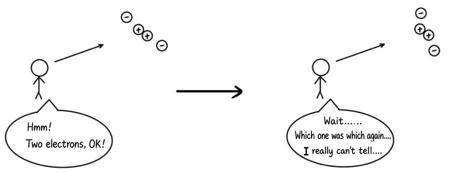
Unlike in classical mechanics, identical particles cannot be distinguished by persistent individual labels in quantum mechanics.

That is why we need the concept of identical particles.

All right, let us begin.

Consider a system composed of two particles.

Let particle 1 occupy the one-particle state

and particle 2 occupy the state

(Wait! I have written these with a lowercase psi because, for now, we are not including spin.

We are considering only the spatial part of the state.

Later, I will use an uppercase Psi for a state function that includes spin, so please keep the uppercase and lowercase Greek letters distinct.

Unfortunately, the old equation editor does not make the difference between uppercase and lowercase psi very obvious.)

Assume here that ψₐ and ψᵦ are distinct, normalized, mutually orthogonal one-particle states. The wave function for the corresponding labeled product is

(Their overlap is S = ⟨ψₐ|ψᵦ⟩ = 0, so the displayed 1/√2 normalization used below applies.)

But did we not just say that we cannot identify which identical particle is which?

We must therefore include the exchanged assignment as well:

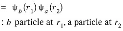
Then

is an equal-amplitude superposition of two orthogonal labeled product components. Each coefficient has squared magnitude one-half, but particle identity is not a separately observable classical alternative.

That is,

For nonorthogonal states with overlap S, the normalization factors are N₊ = 1/√[2(1 + |S|²)] and N₋ = 1/√[2(1 - |S|²)]. If a = b, the antisymmetric combination is identically zero and cannot be normalized.

If this is true, it has an important consequence.

When particles a and b are exchanged, the physical state of the entire system cannot change.

In equation form,

However, quantum mechanics allows another possibility as well:

In some states, the exchange produces a minus sign:

This means

which may look rather mysterious at first.

(You may not yet see what this means—I certainly did not when I first encountered it.

Keep reading to the end, then return to this point; the idea should be much clearer.)

Combining the two possibilities, we can write

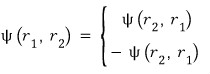
The first is called a symmetric state, with exchange eigenvalue +1,

and the second is called an antisymmetric state, with exchange eigenvalue -1.

Now for the key conclusion.

For two identical bosons, whose spin is an integer, the total state is symmetric under exchange,

whereas for two identical fermions, whose spin is a half-integer, the total state is antisymmetric under exchange.

(Here we will take this spin-statistics connection as an experimentally established fact. We will need it throughout the discussion below,

so please keep it in mind.)

So far, we have discussed only the spatial part of the state.

Now let us include spin.

We will work with two electrons, which are fermions.

(The reason for this choice will soon become clear.)

The state function for the complete two-electron system is

This notation includes both the spatial and spin parts.

We just learned that two electron spins can be combined into four states.

(Remember that we are considering two electrons.)

These are the four spin states—the eigenstates we discussed previously.

Why did I distinguish them with red, blue, and a slash?

The three red states are unchanged when the labels of electrons 1 and 2 are exchanged.

In other words, they are symmetric.

The single blue state acquires a factor of -1 under that exchange.

Because electrons are fermions, the total state function

must be antisymmetric under exchange.

The two allowed spatial-spin pairings are shown below.

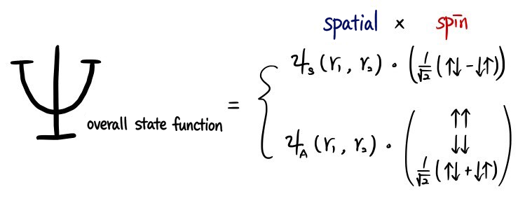
(The subscripts on psi indicate the symmetric and antisymmetric spatial combinations.)

One more important result follows immediately.

It is the familiar Pauli exclusion principle.

Question: what happens if the two electrons are assigned the same spatial orbital?

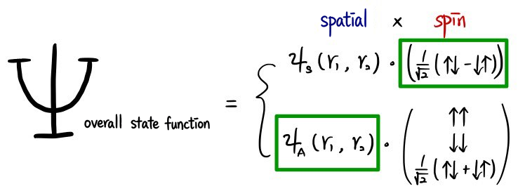
The boxed antisymmetric spatial factor then vanishes, eliminating the complete triplet branch built from it.

The symmetric spatial product paired with the antisymmetric spin singlet does not vanish,

so two opposite-spin electrons may share the same spatial orbital, as the helium 1s² ground state below will show.

Pauli exclusion instead forbids two electrons from occupying the same complete one-electron spin-orbital.

Now we are ready for an appetizer before tackling helium in earnest.

We are about to see why helium is so difficult.

The Hamiltonian for an atom contains

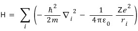
the electrons’ kinetic energy and their electrostatic attraction to the nucleus.

If these were the only terms, helium and heavier atoms would be much easier to solve.

Unfortunately, nature is not so accommodating.

We must add this term:

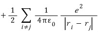
It is the electron-electron repulsion. In most multi-electron atoms, this term prevents an exact analytical solution.

In practical models of solids such as silicon, its many-electron effects are often represented approximately or folded into effective descriptions.

In other systems, including superconductors, electron interactions are essential and cannot simply be neglected.

There are several approximation methods for dealing with such interactions.

But that is not our main subject yet.

(Chapters 6 through 9 will introduce many approximation techniques, so do not worry—we will approximate until we are exhausted.)

Let us continue.

For a Hamiltonian of the form above,

we solve the time-independent Schrödinger equation:

(We can use the time-independent equation here because the potential V has no explicit time dependence.)

We have already treated the one-electron hydrogen atom, so now let us consider helium.

The helium Hamiltonian H is

Because the electron-electron repulsion term is the part that makes the equation difficult,

let us first neglect it and solve the simpler problem.

Once that term is omitted, the system looks like two independent hydrogen-like electrons bound to a nucleus of charge +2e.

We can then write

in this separable form.

(After dropping the electron-electron term, the total Hamiltonian is simply the sum of the Hamiltonians for electrons 1 and 2.)

(It is not literally two hydrogen atoms; it is more like two independent hydrogenic electrons at the same nucleus, each experiencing nuclear charge Z = 2.

That is a useful mental picture, even though calling them two hydrogen atoms would be imprecise.)

In Chapter 4, the energy of an ordinary hydrogen atom was

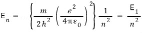
as written here.

For each of the two hydrogenic electrons in our simplified helium model, the ground-state energy is four times the hydrogen value because Z = 2.

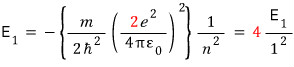
Thus, each electron contributes four times the hydrogen ground-state energy.

Neglecting electron-electron repulsion, the helium ground-state energy is therefore

$E = 4(-13.6 - 13.6)\,\mathrm{eV} = -108.8\,\mathrm{eV} \approx -109\,\mathrm{eV}$

Using a modern reference value, the measured total helium ground-state energy is about -79.0051 eV.

Relative to the model value -108.8 eV, the absolute difference is 29.7949 eV: 37.7126% of the experimental binding-energy magnitude, or 27.3850% of the model magnitude.

This large discrepancy arises primarily from the electron-electron interaction that the independent-particle model neglects.

All right—that completes the first approximation.

Its lesson is simple: helium is hard.

There is another effect that makes the two-electron problem even more interesting.

The expectation value of the repulsion energy depends on whether the spatial state is symmetric or antisymmetric.

This difference is commonly described as the exchange interaction—often called the exchange force in this context, although it is not a new fundamental force.

How does this effective exchange interaction arise?

Before answering, let us introduce orthohelium and parahelium.

We can then return to the exchange interaction itself.

Begin with the ground state of helium.

Saying that helium is in its spatial ground state means

which we will write in this form.

(Again, in this independent-particle approximation, we are still neglecting the electron-electron repulsion.)

Using the Chapter 4 result,

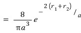
we obtain this spatial wave function.

The spatial part is symmetric under exchange.

Therefore, the spin part of the total fermionic state must be antisymmetric.

In other words, it must be the spin singlet:

Helium whose two electrons have this singlet spin state is called parahelium.

We use the special name because there is another family to compare it with.

That other family is called orthohelium.

The distinction becomes visible in excited states.

Suppose one electron in excited helium occupies the 1,0,0 state while the other occupies an n’,l’,m’ state.

Here we restrict attention to singly excited configurations. Doubly excited helium states can instead autoionize into He⁺ plus an emitted electron or decay radiatively, sometimes populating singly excited neutral states.

The spatial state may then be either symmetric or antisymmetric.

Both possibilities are allowed.

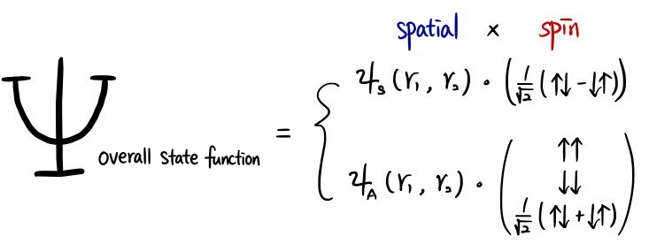
The spin part compensates so that the complete two-electron state remains antisymmetric.

The spin-singlet family is again called parahelium.

The triplet family is called orthohelium.

Why distinguish parahelium from orthohelium if both are helium?

Because their energy levels differ.

For corresponding configurations in this simplified discussion, parahelium has the higher energy and orthohelium the lower energy.

Why?

The exchange interaction provides the explanation.

The corresponding energy difference follows from the direct and exchange integrals.

Here is the central idea.

Exchange interaction:

Symmetric and antisymmetric spatial states produce different electron-electron interaction energies.

A symmetric spatial state gives the electrons a greater probability of being near one another.

Their average electrostatic repulsion is therefore larger, which raises the expectation value of the Hamiltonian.

For the corresponding singlet parahelium state, the energy is consequently higher.

(Let us go over the argument once more.)

1. A symmetric spatial state must be paired with the spin singlet.

2. The spin-singlet helium family is parahelium.

3. A symmetric spatial state gives the electrons a greater probability of being close together.

Their average repulsion is therefore larger,

so the expectation value of the Hamiltonian is higher.

4. In the corresponding comparison, the higher-energy state is parahelium.

For otherwise equivalent noninteracting particles prepared in the same internal or spin state, a symmetric spatial sector produces bunching.

This statistical tendency can resemble an effective attraction,

whereas an antisymmetric spatial sector—such as the electron-triplet sector—produces an exchange hole

and corresponding avoidance that can resemble an effective repulsion. The electron-singlet spatial sector is symmetric and is not covered by that fermion shorthand.

That is where I will conclude Chapter 5.

Many instructors do not cover this topic in an introductory course,

but our professor wanted us to encounter the idea at least once before

moving on to Chapters 6 through 9.

Chapter 5 went by rather quickly, and I still feel as though I am catching my breath.

Next comes Chapter 6: perturbation theory.