Time-Independent Perturbation Theory

This time, we are studying time-independent perturbation theory.

The basic idea is simple: start with a system that we can solve exactly, then ask how its states and energies change when the Hamiltonian is disturbed slightly. I will call the exactly solvable system the unperturbed system and the slightly modified one the perturbed system.

Time-independent perturbation theory is also the natural place to begin before moving on to time-dependent perturbations. It is one of the most useful approximation methods in introductory quantum mechanics, because exactly solvable models are the exception rather than the rule.

From an ideal well to a perturbed system

Recall the infinite square well from the beginning of our study of the time-independent Schrödinger equation:

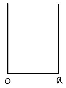
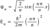
For this ideal system, both the eigenfunctions and eigenvalues are known exactly. To keep the notation clear, I will attach a superscript 0 to every quantity belonging to the unperturbed system:

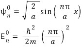
Real systems are rarely this tidy. A more realistic potential might differ from the ideal well by only a small bump:

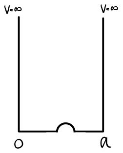
Our goal is to approximate the perturbed eigenfunction and eigenvalue even when the modified Schrödinger equation cannot be solved exactly. That is why perturbation theory is, at heart, an approximation scheme.

Ready? Here we go.

Expansion in the perturbation parameter

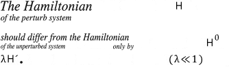
We assume that the perturbed Hamiltonian differs only slightly from the unperturbed Hamiltonian. Introduce a bookkeeping parameter λ and write the perturbation as λH′, with λ much smaller than 1:

$$ H = H^{(0)} + \lambda H'. $$

We make the same kind of expansion for the eigenfunction and eigenvalue:

$$\begin{aligned} |\psi_n\rangle &= |\psi_n^{(0)}\rangle + \lambda |\psi_n^{(1)}\rangle + \lambda^2 |\psi_n^{(2)}\rangle + \cdots, \\ E_n &= E_n^{(0)} + \lambda E_n^{(1)} + \lambda^2 E_n^{(2)} + \cdots. \end{aligned}$$

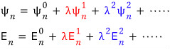
The red terms are the first-order corrections, and the blue terms are the second-order corrections. The superscripts label the order of the approximation; they are not powers. Higher-order terms are progressively suppressed by higher powers of λ.

The exact perturbed state must still satisfy the time-independent Schrödinger equation:

Expand both sides and collect equal powers of λ:

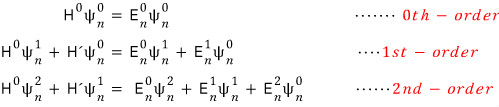
The series could continue to third, fourth, and higher orders. In many weakly perturbed systems, however, the first two corrections already give a useful approximation. We will therefore look for these four quantities:

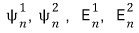
To keep the derivation manageable, this post will not derive the second-order wave-function correction:

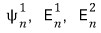
Instead, we will derive the first-order wave-function correction and the first- and second-order energy corrections:

First-order energy correction

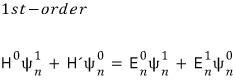
Start with the first-order equation:

$$ H^{(0)}|\psi_n^{(1)}\rangle + H'|\psi_n^{(0)}\rangle = E_n^{(0)}|\psi_n^{(1)}\rangle + E_n^{(1)}|\psi_n^{(0)}\rangle. $$

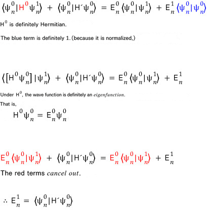
Take the inner product with the unperturbed bra ⟨ψ⁰ₙ|:

Using the Hermiticity of H⁰, its eigenvalue equation, and the normalization of ψ⁰ₙ, the terms containing the first-order state correction cancel, leaving the standard result:

$$ E_n^{(1)} = \langle \psi_n^{(0)}|H'|\psi_n^{(0)}\rangle. $$

So the first of our three targets is complete:

First-order wave-function correction

Now turn to the first-order state correction:

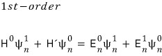
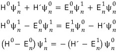
Rearrange the first-order equation:

The unperturbed eigenfunctions form a complete orthonormal basis:

Therefore, any state—including the first-order correction—can be expanded in that basis:

$$ |\psi_n^{(1)}\rangle = \sum_{m\ne n} C_m^{(1)}|\psi_m^{(0)}\rangle. $$

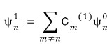
Here, the superscript (1) on the coefficients marks a first-order coefficient. The sum is written over m ≠ n. This corresponds to the conventional intermediate-normalization choice in which the correction has no component parallel to the original state.

This exclusion also prevents the energy denominator that appears below from vanishing. The derivation therefore assumes that E⁰ₙ is nondegenerate; we will treat degeneracy separately later.

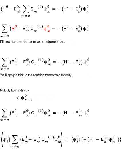
Substitute the basis expansion into the rearranged first-order equation:

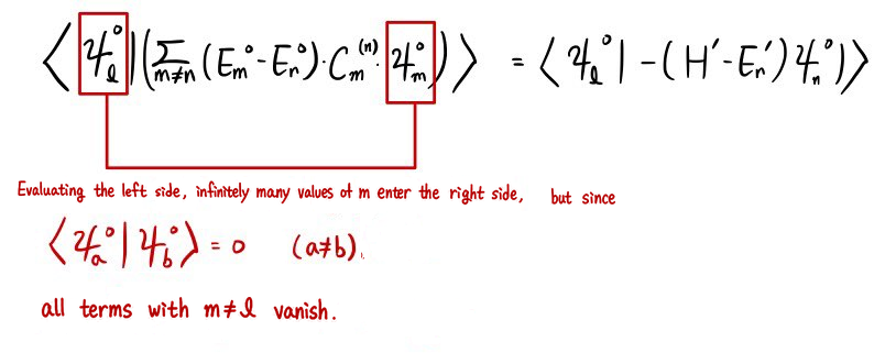
The orthonormality relation isolates one coefficient at a time:

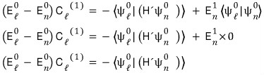
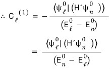
Relabeling the dummy index ℓ as m gives

$$ C_m^{(1)} = \frac{\langle \psi_m^{(0)}|H'|\psi_n^{(0)}\rangle} {E_n^{(0)}-E_m^{(0)}}, \qquad m\ne n. $$

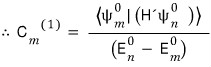
and hence the full first-order wave-function correction:

$$ |\psi_n^{(1)}\rangle = \sum_{m\ne n} \frac{\langle \psi_m^{(0)}|H'|\psi_n^{(0)}\rangle} {E_n^{(0)}-E_m^{(0)}} |\psi_m^{(0)}\rangle. $$

That completes the first-order corrections to both the energy and the state.

Second-order energy correction

The second-order equation is

$$H^{(0)}|\psi_n^{(2)}\rangle + H'|\psi_n^{(1)}\rangle = E_n^{(0)}|\psi_n^{(2)}\rangle + E_n^{(1)}|\psi_n^{(1)}\rangle + E_n^{(2)}|\psi_n^{(0)}\rangle.$$

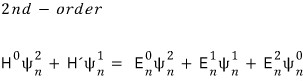
Take its inner product with ⟨ψ⁰ₙ|, just as before:

Hermiticity, normalization, and orthogonality reduce the equation to an expectation value involving the first-order state correction:

$$ E_n^{(2)} = \langle \psi_n^{(0)}|H'|\psi_n^{(1)}\rangle. $$

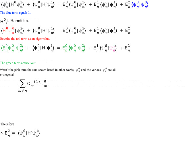
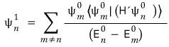
Now substitute the first-order correction found above. The source raster previously shown at this point ended every summand with $|\psi_n^{(0)}\rangle$, even though the summation index is $m$. That subscript is a source error: the basis ket must be $|\psi_m^{(0)}\rangle$. The corrected equation is

$$ |\psi_n^{(1)}\rangle = \sum_{m\ne n} \frac{\langle \psi_m^{(0)}|H'|\psi_n^{(0)}\rangle} {E_n^{(0)}-E_m^{(0)}} |\psi_m^{(0)}\rangle. $$

The retained raster below shows the same corrected ordering, with each basis ket placed before its scalar coefficient:

Substitution gives

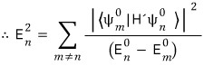
The energy denominator depends on $m$, so it must remain inside the summation. A source raster previously shown here incorrectly moved that denominator outside the sum and then treated a quotient of sums as a sum of termwise quotients. Replacing that invalid step with the correct linearity of the inner product gives

$$ \begin{aligned} E_n^{(2)} &= \left\langle \psi_n^{(0)} \middle| H' \middle| \psi_n^{(1)} \right\rangle \\ &= \sum_{m\ne n} \frac{ \langle \psi_n^{(0)}|H'|\psi_m^{(0)}\rangle \langle \psi_m^{(0)}|H'|\psi_n^{(0)}\rangle }{E_n^{(0)}-E_m^{(0)}}. \end{aligned} $$

Because H′ is Hermitian, the numerator is the squared magnitude of the off-diagonal matrix element:

$$ E_n^{(2)} = \sum_{m\ne n} \frac{\left|\langle \psi_m^{(0)}|H'|\psi_n^{(0)}\rangle\right|^2} {E_n^{(0)}-E_m^{(0)}}. $$

It is convenient to abbreviate a perturbation matrix element as

$$ H'_{ij} \equiv \langle \psi_i^{(0)}|H'|\psi_j^{(0)}\rangle. $$

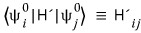
Once H′ and the unperturbed states are known, these matrix elements determine the correction.

Degenerate perturbation theory

What changes if two different unperturbed states have the same energy? Begin with a twofold degeneracy:

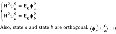
Any linear combination of those two states is also an eigenstate of H⁰ with the same eigenvalue:

$$ |\psi^{(0)}\rangle = \alpha|\psi_a^{(0)}\rangle + \beta|\psi_b^{(0)}\rangle. $$

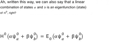
So write the unperturbed state as that linear combination, then expand the Hamiltonian, state, and energy as before:

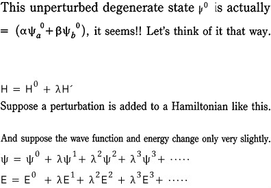
Substitution into the Schrödinger equation again gives the perturbative hierarchy:

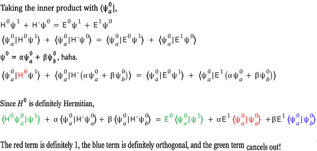
At first order,

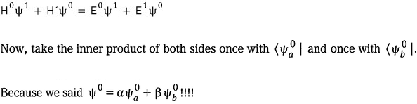
projecting onto ⟨ψ⁰ₐ| gives one linear equation for α and β:

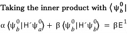
Projecting onto ⟨ψ⁰_b| gives the second equation:

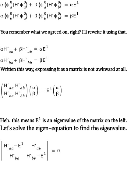
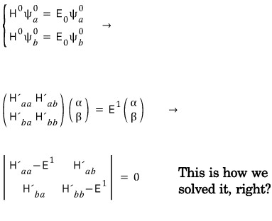
Together, the two equations form a matrix eigenvalue problem inside the degenerate subspace:

$$ \begin{pmatrix} H'_{aa} & H'_{ab} \\ H'_{ba} & H'_{bb} \end{pmatrix} \begin{pmatrix}\alpha\\\beta\end{pmatrix} = E^{(1)} \begin{pmatrix}\alpha\\\beta\end{pmatrix}, \qquad \det\!\begin{pmatrix} H'_{aa}-E^{(1)} & H'_{ab} \\ H'_{ba} & H'_{bb}-E^{(1)} \end{pmatrix}=0. $$

The allowed first-order corrections are the eigenvalues of that matrix:

$$ E_{\pm}^{(1)} = \frac{H'_{aa}+H'_{bb}}{2} \pm \frac{1}{2} \sqrt{\left(H'_{aa}-H'_{bb}\right)^2+4|H'_{ab}|^2}. $$

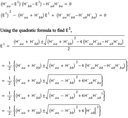
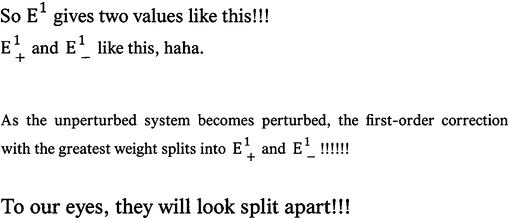
Thus, a twofold degenerate level generally splits into two first-order levels:

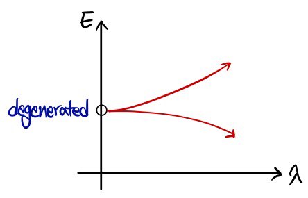
That is the central lesson of degenerate perturbation theory: before using the nondegenerate formulas, diagonalize H′ within the degenerate subspace.

For twofold degeneracy, the calculation can be summarized as follows:

For an r-fold degeneracy, the same idea becomes an r-dimensional eigenvalue equation:

$$ \sum_{j=1}^{r}\left(H'_{ij}-E^{(1)}\delta_{ij}\right)c_j=0 \quad (i=1,\ldots,r), \qquad \det\!\left(H'-E^{(1)}I_r\right)=0. $$

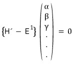
Solve that eigenvalue problem to obtain the first-order energy shifts and the correct linear combinations of unperturbed states. We will save worked examples of higher-order degeneracy for another post.

Whew—that was a long one, but the theory is finally in place.