Spin-Orbit Coupling (LS Coupling) and the Fine Structure of Hydrogen

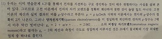
OK so — whether we’re talking about an electron or a proton, both have spin. And the magnetic moment that comes from spin is inversely proportional to mass.

Meaning: the electron’s spin magnetic moment is waaaaaay more dominant than the proton’s.

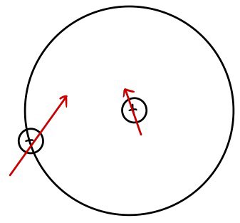
So here’s what we’re going to do. Flip the reference frame. Instead of picturing the electron orbiting the proton, we’ll picture the proton orbiting the electron. That’s our new point of view.

From the electron’s seat, we can draw a picture like this: proton going around → current → magnetic field, plus the electron’s own spin sitting in that field.

The Hamiltonian for this, same move as before, is

$$H_{spin-orbit}^{'} = -\overrightarrow{\mu}\cdot\overrightarrow{B}$$

And this is an energy we’d been completely ignoring up to now.

What does it actually mean though?

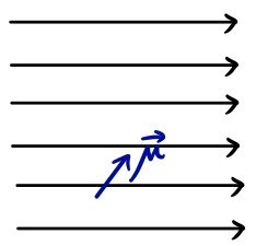
If you drop a magnetic moment inside a B field, a force kicks in that tries to align $\mu$ with $B$. (Because that’s the direction total energy goes down, and lowest-energy = most stable state.) So the system shifts toward whichever side makes the energy smaller.

Can we then call this Hamiltonian the 1st correction?????

Let’s call it the 1st correction. And to actually compute it, let’s find $\mu$ and $B$ separately.

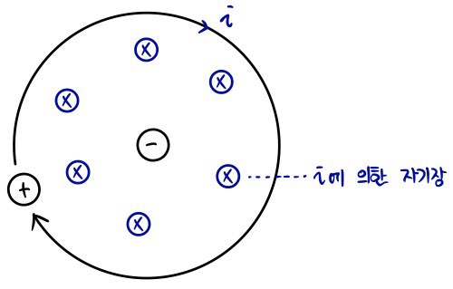
$B$ is easy — Biot–Savart has us covered:

$$\text{Biot-Savart's law} \\ \overrightarrow{B} = \frac{\mu_{0}}{4\pi}\int\frac{I\cdot d\overrightarrow{\ell}\times\hat{\eta}}{\eta^{2}} \\ \text{Since }d\overrightarrow{\ell}\text{ and }\hat{\eta}\text{ are always }90^\circ\text{, and since we are finding the magnetic field felt by the electron, }\eta = r \\ \hat{h}\text{ unit vector in the direction of the cross product vector (angular momentum vector direction)} \\ = \frac{\mu_{0}}{4\pi}\int\frac{I\cdot d\ell}{r^{2}}\hat{h} = \frac{\mu_{0}}{4\pi}I\frac{2\pi r}{r^{2}}\hat{h} = \frac{\mu_{0}I}{2r}\hat{h} \\ I = \frac{dQ}{dt} = \frac{e}{T} = \frac{e}{2\pi r/v}\text{, and} \\ \text{therefore, }\overrightarrow{B} = \frac{\mu_{0}}{2r}\frac{e}{2\pi r/v}\hat{h} = \frac{\mu_{0}}{4\pi r^{2}}ev\hat{h} \\ \text{The red combination can be written as }\overrightarrow{L}\text{. Because }m\overrightarrow{v}\times\overrightarrow{r} = \overrightarrow{L} = L\hat{h} \\ \text{i.e., }\overrightarrow{B} = \frac{\mu_{0}}{4\pi r^{2}}ev\hat{h} = \frac{\mu_{0}}{4\pi r^{2}}e\frac{mvr}{mr}\hat{h} = \frac{\mu_{0}e}{4\pi mr^{3}}\overrightarrow{L} \\ \text{If we mess around a bit more with }c = \frac{1}{\sqrt{\mu_{0}\epsilon_{0}}}\text{ — let's mess.} \\ \overrightarrow{B} = \frac{\mu_{0}e}{4\pi mr^{3}}\overrightarrow{L} = \frac{\mu_{0}\epsilon_{0}e}{4\pi\epsilon_{0}mr^{3}}\overrightarrow{L} = \frac{e}{4\pi\epsilon_{0}c^{2}mr^{3}}\overrightarrow{L}$$

OK, B — done.

Now mu. And this is where the pain starts……(sobbing)

$$\text{Definition of }\overrightarrow{\mu}\text{: current times area vector! } = I\overrightarrow{A} \\ I = \frac{dQ}{dt} = \frac{-e}{T}\quad(\text{since it's the electron's }\mu\text{, we get }{-e}) \\ \text{so, }\overrightarrow{\mu} = -\frac{e}{T}\overrightarrow{A} \\ \text{And this }\overrightarrow{\mu}\text{ should be proportional to }\overrightarrow{S}. \\ \overrightarrow{\mu} = \gamma\overrightarrow{S} \\ (\text{The gamma-finding game begins.}) \\ \text{So }{-\frac{e}{T}\overrightarrow{A}} = \gamma\overrightarrow{S} \\ \text{I'll only track magnitudes.}\quad -\frac{e\pi r^{2}}{T} = \gamma S$$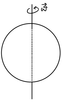

Whatever, I give up. Let’s just pretend the electron is a sphere.

The angular momentum of a sphere — $S = I\omega$.

$I$ is the moment of inertia, and for a sphere $I = mr^{2}$!!!

And $\omega = 2\pi/T$, so

$$-\frac{e\pi r^{2}}{T} = \gamma S = \gamma Iw = \gamma\left(mr^{2}\right)\frac{2\pi}{T} \\ \therefore\quad\gamma = -\frac{e}{2m}$$

Oh — that came out super easy!!!!!!

$$\overrightarrow{\mu_{e}}\quad:\quad\text{magnetic moment of the electron} \\ \overrightarrow{\mu_{e}} = -\frac{e}{2m}\overrightarrow{S}$$

Easy, right!!!! Isn’t it?!?!? Of course it’s easy!!!!

Because…

It’s wrong!!!!!!!!!!!! lmao lmao lmao

Why it’s wrong:

1. The electron is not a sphere.

2. You can’t just plug in classical velocities — the electron’s orbital speed, its “rotational” speed, none of that. There are relativistic effects, so it has to be done properly with relativistic quantum mechanics. That’s the TL;DR.

When you actually grind through it with relativistic QM, the answer comes out exactly twice as large.

$$\therefore\quad\overrightarrow{\mu_{e}} = -\frac{e}{m}\overrightarrow{S}$$

Dirac was apparently the first to nail this down.

(Whether I’ll ever actually cover relativistic QM on this blog… honestly, I don’t know… T_T T_T T_T ha… I’ll at least leave a footnote.)

Not that shocking, really. There are tons of things undergrads can’t derive from scratch, so — welcome to the club :)

OK so — shall we finally compute the Hamiltonian???

$$H_{so}^{'} = -\overrightarrow{\mu}\cdot\overrightarrow{B} = -\left(-\frac{e}{m}\overrightarrow{S}\right)\left(\frac{e}{4\pi\epsilon_{0}c^{2}mr^{3}}\overrightarrow{L}\right) = \frac{e^{2}}{4\pi\epsilon_{0}c^{2}m^{2}r^{3}}\overrightarrow{S}\cdot\overrightarrow{L}$$

BUT — we have to multiply this by $1/2$.

Quick version: we’re currently looking at everything from the electron’s rest frame, and to cancel out that choice of frame, a $1/2$ has to come in. This is called the Thomas correction.

It’s a tough concept;;;;

Leaving a footnote.

Footnote:

One way to think about the $1/2$: picture the electron constantly hopping from one inertial frame to the next. The correction is basically the sum of all the Lorentz transformations you’d need as the frame keeps shifting.

To dodge this whole mess, you could do everything in the rest frame of the nucleus — in that frame, the proton produces only an electric field. Then you’d ask: how can a pure electric field exert a torque on the electron?

The key fact is that a moving magnetic dipole also picks up an electric dipole moment. So in that frame, spin-orbit coupling shows up as the interaction between the nucleus’s electric field and the electron’s magnetic moment.

But that analysis is way messier, which is why we did it in the electron’s rest frame in the main text. Only then does the physics actually stay clean.

$$\therefore\quad H_{so}^{'} = \frac{e^{2}}{8\pi\epsilon_{0}c^{2}m^{2}r^{3}}\overrightarrow{S}\cdot\overrightarrow{L}$$

So roughly — once we actually consider spin and orbit together, we get an error of about this much compared to pretending it wasn’t there.

(It’s pretty rough, yeah.)

A little handwavy in spots, but — we have our Hamiltonian correction.

But then another problem shows up. With the eigenfunctions we currently have, we can’t actually compute the expectation value of this Hamiltonian.

$$\text{Sure, with }\psi_{n,l,m}^{0}\text{ we can grab stuff like }L^{2},\quad S^{2}, \\ \text{but }L\cdot S\text{? Nope.} \\ \text{Because }\psi_{n,l,m}^{0}\text{ isn't an eigenfunction of }L\cdot S.$$$$E_{so}^{1} = \left<\psi_{n,l,m}^{0}\middle|H_{so}^{'}\middle|\psi_{n,l,m}^{0}\right> = \left<\psi_{n,l,m}^{0}\middle|\frac{e^{2}}{8\pi\epsilon_{0}c^{2}m^{2}r^{3}}\overrightarrow{S}\cdot\overrightarrow{L}\middle|\psi_{n,l,m}^{0}\right>$$

And this is exactly our current situation!!

So — we define a new angular momentum. Then everything unlocks.

$$J = L + S$$

Define that as the total angular momentum vector, and we can finally get the expectation value of $L\cdot S$.

Because

$$L^{2},\quad S^{2},\quad J^{2}$$

these can all be measured simultaneously, and

$$J^{2} = \left(L + S\right)\left(L + S\right) = L^{2} + S^{2} + 2L\cdot S \\ L\cdot S = \frac{1}{2}\left\{J^{2} - L^{2} - S^{2}\right\}$$

So since we need to measure $L\cdot S$ this way, we’re going to swap out our quantum numbers $n, l, m, s, m_{s}$!!

Replace the eigenfunction with quantum numbers $n, l, s, j, m_{j}$, and now $L\cdot S$ is covered too.

Then the 1st correction becomes — courtesy of swapping quantum numbers!!! —

$$E_{so}^{1} = \left<\psi_{n,l,s,j,m_{j}}^{0}\middle|H_{so}^{'}\middle|\psi_{n,l,s,j,m_{j}}^{0}\right> \\ = \left<\psi_{n,l,s,j,m_{j}}^{0}\middle|\frac{e^{2}}{8\pi\epsilon_{0}c^{2}m^{2}r^{3}}\overrightarrow{S}\cdot\overrightarrow{L}\middle|\psi_{n,l,s,j,m_{j}}^{0}\right> \\ = \left<\psi_{n,l,s,j,m_{j}}^{0}\middle|\frac{e^{2}}{4\pi\epsilon_{0}c^{2}m^{2}r^{3}}\left(J^{2} - L^{2} - S^{2}\right)\middle|\psi_{n,l,s,j,m_{j}}^{0}\right>$$

Since $J$ is angular momentum, it obeys every angular-momentum rule we’ve already figured out. (Spin worked by the exact same logic, right?)

Which is to say:

$$\text{The eigenvalue of }\frac{1}{2}\left\{J^{2} - L^{2} - S^{2}\right\}\text{ is }\frac{\hbar^{2}}{2}\left\{j(j+1) - \ell(\ell+1) - s(s+1)\right\}. \\ \text{That's the point.} \\ \text{Plugging into the expression above:}$$$$E_{so}^{1} = \left<\psi_{n,l,s,j,m_{j}}^{0}\middle|\frac{e^{2}}{4\pi\epsilon_{0}c^{2}m^{2}r^{3}}\left(J^{2} - L^{2} - S^{2}\right)\middle|\psi_{n,l,s,j,m_{j}}^{0}\right> \\ = \frac{e^{2}}{8\pi\epsilon_{0}c^{2}m^{2}}\frac{\hbar^{2}}{2}\left\{j(j+1) - \ell(\ell+1) - s(s+1)\right\}\left<\frac{1}{r^{3}}\right>$$

And what’s left to actually compute is the expectation value of $1/r^{3}$.

Which — we already proved, last post!!!!

(http://gdpresent.blog.me/220577832479)

Quantum mechanics I studied #29. Kramer’s relation (Kramers’ relation)

(Mr. Isaac Newton who invented calculus hehehehehehe)(If someone builds a time machine, he’s target number one…

blog.naver.com

$$\left<\frac{1}{r^{3}}\right> = \frac{1}{\ell\left(\ell + \frac{1}{2}\right)\left(\ell + 1\right)n^{3}a^{3}}$$

That was it.

So:

$$E_{so}^{1} = \frac{e^{2}}{8\pi\epsilon_{0}c^{2}m^{2}}\frac{\hbar^{2}}{2}\left\{j(j+1) - \ell(\ell+1) - s(s+1)\right\}\left<\frac{1}{r^{3}}\right> \\ = \frac{e^{2}}{8\pi\epsilon_{0}c^{2}m^{2}}\frac{\hbar^{2}}{2}\left\{j(j+1) - \ell(\ell+1) - s(s+1)\right\}\frac{1}{\ell\left(\ell + \frac{1}{2}\right)\left(\ell + 1\right)n^{3}a^{3}} \\ = \frac{e^{2}}{8\pi\epsilon_{0}c^{2}m^{2}}\frac{\hbar^{2}}{2}\frac{\left\{j(j+1) - \ell(\ell+1) - s(s+1)\right\}}{\ell\left(\ell + \frac{1}{2}\right)\left(\ell + 1\right)n^{3}a^{3}} \\ = \frac{E_{n}^{2}}{m_{0}c^{2}}\frac{\left\{j(j+1) - \ell(\ell+1) - \frac{3}{4}\right\}n}{\ell\left(\ell + \frac{1}{2}\right)\left(\ell + 1\right)}$$

And that’s how we land the energy correction from LS coupling.

The fine structure — that’s the name for the hydrogen atom’s structure once you bundle the relativistic correction and the LS coupling correction together.

And as I mentioned earlier — we’re talking an energy correction on the order of about $1/10000$!!

---

Originally written in Korean on my Naver blog (2015-12). Translated to English for gdpark.blog.