Van der Waals Interaction and the Stark Effect
Turns out neutral atoms *do* attract each other — we Taylor-expand the Coulomb mess in Griffiths 6.31 to derive the Van der Waals interaction using perturbation theory.
Prob 6.31
Two atoms, separated by distance $R$. They’re electrically neutral, so your first instinct is: no force between them, right? Wrong — if they can be polarized, there’s actually a weak attractive force between them.
To model this (Figure 6.14), draw each atom as an electron (charge $-e$) connected by a spring (spring constant $k$) to a nucleus (charge $+e$). Assume the nucleus is heavy and basically doesn’t move.
The unperturbed Hamiltonian:
$$H^{0} = \frac{p_{1}^{2}}{2m} + \frac{1}{2}kx_{1}^{2} + \frac{p_{2}^{2}}{2m} + \frac{1}{2}kx_{2}^{2}$$And the Coulomb interaction between the atoms:
$$H' = \frac{1}{4\pi\epsilon_{0}}\left(\frac{e^{2}}{R} - \frac{e^{2}}{R-x_{1}} - \frac{e^{2}}{R-x_{2}} + \frac{e^{2}}{R+x_{1}-x_{2}}\right)$$a) Assuming $|x_1|, |x_2| \ll R$, show:
$$H' \cong -\frac{e^{2}x_{1}x_{2}}{2\pi\epsilon_{0}R^{3}}$$OK so — start from:
$$H' = \frac{1}{4\pi\epsilon_{0}}\left(\frac{e^{2}}{R} - \frac{e^{2}}{R-x_{1}} - \frac{e^{2}}{R+x_{2}} + \frac{e^{2}}{R-x_{1}+x_{2}}\right)$$Time to Taylor-expand the perturbation. Quick reminders:
$$\begin{aligned} &* \quad (1+x)^{n} = 1 + nx + \frac{n(n-1)}{2!}x^{2} + \cdots \\ &* \quad (1-x)^{-1} = 1 + x + x^{2} + \cdots \\ &* \quad (1-(-x))^{-1} = 1 - x + x^{2} - \cdots \end{aligned}$$Plug and chug:
$$\begin{aligned} H' &= \frac{1}{4\pi\epsilon_{0}}\left(\frac{e^{2}}{R} - \frac{e^{2}}{R-x_{1}} - \frac{e^{2}}{R+x_{2}} + \frac{e^{2}}{R+x_{1}-x_{2}}\right) \\ &= \frac{e^{2}}{4\pi\epsilon_{0}}\left(\frac{1}{R} - \frac{1}{R}\frac{1}{\left(1-\frac{x_{1}}{R}\right)} - \frac{1}{R}\frac{1}{\left(1+\frac{x_{2}}{R}\right)}\right) \end{aligned}$$$$\begin{aligned} H' &= \frac{1}{4\pi\epsilon_{0}}\left(\frac{e^{2}}{R} - \frac{e^{2}}{R-x_{1}} - \frac{e^{2}}{R+x_{2}} + \frac{e^{2}}{R+x_{1}-x_{2}}\right) \\ &= \frac{e^{2}}{4\pi\epsilon_{0}}\left(\frac{1}{R} - \frac{1}{R}\frac{1}{\left(1-\frac{x_{1}}{R}\right)} - \frac{1}{R}\frac{1}{\left(1+\frac{x_{2}}{R}\right)} + \frac{1}{R}\frac{1}{1-\frac{(x_{1}-x_{2})}{R}}\right) \\ &= \frac{e^{2}}{4\pi\epsilon_{0}R}\left(1 - \left(1-\frac{x_{1}}{R}\right)^{-1} - \left(1+\frac{x_{2}}{R}\right)^{-1} + \left(1-\frac{(x_{1}-x_{2})}{R}\right)^{-1}\right) \\ &\cong \frac{e^{2}}{4\pi\epsilon_{0}R}\left(1 - \left(1+\frac{x_{1}}{R}+\left(\frac{x_{1}}{R}\right)^{2}+\cdots\right) - \left(1-\frac{x_{2}}{R}+\left(\frac{x_{2}}{R}\right)^{2}-\cdots\right) + \left(1+\frac{x_{1}-x_{2}}{R}+\left(\frac{x_{1}-x_{2}}{R}\right)^{2}+\cdots\right)\right) \end{aligned}$$$$\begin{aligned} &\cong \frac{e^{2}}{4\pi\epsilon_{0}R}\left(1 - 1 - \frac{x_{1}}{R} - \frac{x_{1}^{2}}{R^{2}} - 1 + \frac{x_{2}}{R} - \frac{x_{2}^{2}}{R^{2}} + 1 + \frac{x_{1}-x_{2}}{R} + \frac{(x_{1}-x_{2})^{2}}{R^{2}}\right) \\ &\cong \frac{e^{2}}{4\pi\epsilon_{0}R}\left(-\frac{(x_{1}-x_{2})}{R} - \frac{(x_{1}^{2}+x_{2}^{2})}{R^{2}} + \frac{(x_{1}-x_{2})}{R} + \frac{x_{1}^{2}-2x_{1}x_{2}+x_{2}^{2}}{R^{2}}\right) \\ &\cong \frac{e^{2}}{4\pi\epsilon_{0}R}\left(\frac{-2x_{1}x_{2}}{R^{2}}\right) = -\frac{e^{2}x_{1}x_{2}}{2\pi\epsilon_{0}R^{3}} \end{aligned}$$Whoa. Look at that cancellation. How clean is that?!
b) Show that the total Hamiltonian splits into two harmonic oscillators:
$$H = \left[\frac{1}{2m}p_{+}^{2} + \frac{1}{2}\left(k - \frac{e^{2}}{4\pi\epsilon_{0}R^{3}}\right)x_{+}^{2}\right] + \left[\frac{1}{2m}p_{-}^{2} + \frac{1}{2}\left(k - \frac{e^{2}}{4\pi\epsilon_{0}R^{3}}\right)x_{-}^{2}\right]$$with the change of variables:
$$x_{\pm} \equiv \frac{1}{\sqrt{2}}\left(x_{1} \pm x_{2}\right), \qquad p_{\pm} \equiv \frac{1}{\sqrt{2}}\left(p_{1} \pm p_{2}\right)$$What we have so far:
$$\begin{aligned} H &= H^{0} + H' \\ &= \frac{p_{1}^{2}}{2m} + \frac{1}{2}kx_{1}^{2} + \frac{p_{2}^{2}}{2m} + \frac{1}{2}kx_{2}^{2} - \frac{e^{2}}{2\pi\epsilon_{0}R^{3}}x_{1}x_{2} \end{aligned}$$So basically they’re telling us: do a change of variables, the thing falls apart into two independent oscillators. Just substitute. Carefully.
Invert the change of variables:
$$\begin{aligned} x_{+} &= \frac{1}{\sqrt{2}}x_{1} + \frac{1}{\sqrt{2}}x_{2} \quad \to \quad \sqrt{2}x_{+} = x_{1} + x_{2} \\ x_{-} &= \frac{1}{\sqrt{2}}x_{1} - \frac{1}{\sqrt{2}}x_{2} \quad \to \quad \sqrt{2}x_{-} = x_{1} - x_{2} \\ &\to \quad \therefore \quad x_{1} = \frac{\sqrt{2}}{2}x_{+} + \frac{\sqrt{2}}{2}x_{-} \\ &\to \quad \therefore \quad x_{2} = \frac{\sqrt{2}}{2}x_{+} - \frac{\sqrt{2}}{2}x_{-} \end{aligned}$$$p_+$ and $p_-$ are the exact same flavor of object, so by the same logic:
$$\begin{aligned} &p_{1} = \frac{\sqrt{2}}{2}p_{+} + \frac{\sqrt{2}}{2}p_{-} \\ &p_{2} = \frac{\sqrt{2}}{2}p_{+} - \frac{\sqrt{2}}{2}p_{-} \end{aligned}$$Yeah, that should be right.
Now sub into the Hamiltonian:
$$\begin{aligned} H &= H^{0} + H' \\ &= \frac{p_{1}^{2}}{2m} + \frac{1}{2}kx_{1}^{2} + \frac{p_{2}^{2}}{2m} + \frac{1}{2}kx_{2}^{2} - \frac{e^{2}}{2\pi\epsilon_{0}R^{3}}x_{1}x_{2} \end{aligned}$$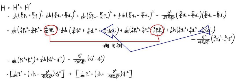
Wait — is the problem wrong? Why am I getting this?
Collecting the harmonic-oscillator-looking pieces into $\tfrac{1}{2}kx^2$ form:
$$= \left[\frac{1}{2m}p_{+}^{2} + \frac{1}{2}\left(k - \frac{e^{2}}{2\pi\epsilon_{0}R^{3}}\right)x_{+}^{2}\right] + \left[\frac{1}{2m}p_{-}^{2} + \frac{1}{2}\left(k + \frac{e^{2}}{2\pi\epsilon_{0}R^{3}}\right)x_{-}^{2}\right]$$So the Hamiltonian is really just two harmonic oscillators glued together, with effective spring constants:
$$k' = k - \frac{e^{2}}{2\pi\epsilon_{0}R^{3}}, \qquad k'' = k + \frac{e^{2}}{2\pi\epsilon_{0}R^{3}}$$Next — the ground state energy
Two independent oscillators, so obviously:
$$E = \frac{1}{2}\hbar(\omega_{+} + \omega_{-}), \qquad \omega_{\pm} = \sqrt{\frac{k \mp e^{2}/2\pi\epsilon_{0}R^{3}}{m}}$$With no Coulomb interaction at all:
$$E_{0} = \hbar\omega_{0}, \qquad \omega_{0} = \sqrt{\frac{k}{m}}$$Now assuming $k \gg e^{2}/2\pi\epsilon_{0}R^{3}$, show:
$$\Delta V = E - E_{0} \simeq -\frac{\hbar}{8m^{2}\omega_{0}^{3}}\left(\frac{e^{2}}{4\pi\epsilon_{0}}\right)^{2}\frac{1}{R^{6}}$$I’ll read this as: find the energy difference between perturbed and unperturbed, and go.
$$\begin{aligned} E &= \frac{\hbar}{2}(\omega_{+} + \omega_{-}) = \frac{\hbar}{2}\left\{\sqrt{\frac{k-e^{2}/2\pi\epsilon_{0}R^{3}}{m}} + \sqrt{\frac{k+e^{2}/2\pi\epsilon_{0}R^{3}}{m}}\right\} \\ &= \frac{\hbar}{2}\left\{\sqrt{\frac{k}{m}-\frac{e^{2}/2\pi\epsilon_{0}R^{3}}{m}} + \sqrt{\frac{k}{m}+\frac{e^{2}/2\pi\epsilon_{0}R^{3}}{m}}\right\} \\ &= \frac{\hbar}{2}\left\{\sqrt{\frac{k}{m}\left(1-\frac{e^{2}}{2\pi\epsilon_{0}R^{3}k}\right)} + \sqrt{\frac{k}{m}\left(1+\frac{e^{2}}{2\pi\epsilon_{0}R^{3}k}\right)}\right\} \\ &= \frac{\hbar}{2}\left\{\sqrt{\omega_{0}^{2}\left(1-\frac{e^{2}}{2\pi\epsilon_{0}R^{3}k}\right)} + \sqrt{\omega_{0}^{2}\left(1+\frac{e^{2}}{2\pi\epsilon_{0}R^{3}k}\right)}\right\} \\ &= \frac{\hbar\omega_{0}}{2}\left\{\left(1-\frac{e^{2}}{2\pi\epsilon_{0}R^{3}k}\right)^{\frac{1}{2}} + \left(1+\frac{e^{2}}{2\pi\epsilon_{0}R^{3}k}\right)^{\frac{1}{2}}\right\} \end{aligned}$$Those little things in the parentheses? They’re extremely small. That’s the hint — Taylor expand.
And we have to keep terms all the way up to 3rd order. Why? Because the 1st-order corrections smash together and die — they cancel. So if we stop too early, we get zero and nothing interesting happens.
$$\begin{aligned} &\cong \frac{\hbar\omega_{0}}{2}\left\{\left(1 - \frac{1}{2}\left(\frac{e^{2}}{2\pi\epsilon_{0}R^{3}k}\right) - \frac{1}{8}\left(\frac{e^{2}}{2\pi\epsilon_{0}R^{3}k}\right)^{2} + \cdots\right) + \left(1 + \frac{1}{2}\left(\frac{e^{2}}{2\pi\epsilon_{0}R^{3}k}\right) - \frac{1}{8}\left(\frac{e^{2}}{2\pi\epsilon_{0}R^{3}k}\right)^{2} + \cdots\right)\right\} \\ &\cong \frac{\hbar\omega_{0}}{2}\left\{2 - \frac{1}{4}\left(\frac{e^{2}}{2\pi\epsilon_{0}R^{3}k}\right)^{2}\right\} = \hbar\omega_{0} - \frac{1}{8}\hbar\omega_{0}\left(\frac{e^{2}}{2\pi\epsilon_{0}R^{3}k}\right)^{2} \end{aligned}$$And now the subtraction:
$$\begin{aligned} \therefore \quad E - E_{0} &= \hbar\omega_{0} - \frac{1}{8}\hbar\omega_{0}\left(\frac{e^{2}}{2\pi\epsilon_{0}R^{3}k}\right)^{2} - \hbar\omega_{0} \\ &= -\frac{1}{8}\hbar\omega_{0}\left(\frac{e^{2}}{2\pi\epsilon_{0}R^{3}k}\right)^{2} \\ &= -\frac{\hbar\omega_{0}}{8}\frac{1}{k^{2}}\left(\frac{e^{2}}{2\pi\epsilon_{0}}\right)^{2}\frac{1}{R^{6}} \end{aligned}$$And since $\omega_0 = \sqrt{k/m}$, rewrite $k^2$ as $m^2\omega_0^4$:
$$= -\frac{\hbar\omega_{0}}{8}\frac{1}{m^{2}\omega_{0}^{4}}\left(\frac{e^{2}}{2\pi\epsilon_{0}}\right)^{2}\frac{1}{R^{6}} = -\frac{\hbar}{8m^{2}\omega_{0}^{3}}\left(\frac{e^{2}}{2\pi\epsilon_{0}}\right)^{2}\frac{1}{R^{6}}$$Prob 6.36
Put an atom in a constant external electric field $E_{ext}$ and its energy levels shift. That’s the Stark effect — basically the electric-field cousin of the Zeeman effect.
In this problem we look at the Stark effect for the $n=1$ and $n=2$ states of hydrogen.
If the field points along $z$, the electron’s potential energy is:
$$\begin{aligned} H_{s}^{'} &= eE_{ext}z \\ &= eE_{ext}r\cos\theta \end{aligned}$$Treat this as a perturbation to the Bohr Hamiltonian $\left(H = -\frac{\hbar^{2}}{2m}\nabla^{2} - \frac{e^{2}}{4\pi\epsilon_{0}}\frac{1}{r}\right)$.
(Spin doesn’t matter here, so ignore it. Same with hyperfine structure.)
a) Show the ground state energy isn’t shifted at first order.
We proved in Chapter 4 that $\psi_{1,0,0} = \frac{1}{\sqrt{\pi a^{3}}}e^{-r/a}$.
$$\begin{aligned} E_{s}^{1} &= \langle\psi_{1,0,0}|eE_{ext}r\cos\theta|\psi_{1,0,0}\rangle \\ &= \int \left(\frac{1}{\sqrt{\pi a^{3}}}e^{-\frac{r}{a}}\left(eE_{ext}r\cos\theta\right)\frac{1}{\sqrt{\pi a^{3}}}e^{-\frac{r}{a}}\right)dV \\ &= \frac{e}{\pi a^{3}}E_{ext}\int\left(e^{-\frac{2r}{a}}r\cos\theta\right)r^{2}\sin\theta\, dr\, d\theta\, d\varphi \end{aligned}$$Pull out the $d\varphi$ integral:
$$\begin{aligned} &= \frac{2\pi e}{\pi a^{3}}E_{ext}\int\left(e^{-\frac{2r}{a}}r\cos\theta\right)r^{2}\sin\theta\, dr\, d\theta \\ &= \frac{2e}{a^{3}}E_{ext}\left\{\left(\int_{0}^{\infty}e^{-\frac{2r}{a}}r^{3}\,dr\right)\left(\int_{0}^{\pi}\frac{1}{2}\sin\theta\, d\theta\right)\right\} \end{aligned}$$Wait — look at the $\theta$ integral. $\int_0^{\pi} \tfrac{1}{2}\sin\theta\cos\theta\,d\theta = 0$. That’s the killer. The $\cos\theta$ zeroes it out.
$$\therefore \quad E_{s}^{1} = 0$$b) The first excited state — 4-fold degenerate.
$$\psi_{2,0,0}, \quad \psi_{2,1,1}, \quad \psi_{2,1,0}, \quad \psi_{2,1,-1}$$Use degenerate perturbation theory to find the first-order correction. How many levels does $E_2$ split into?
Back in the two-fold degenerate case, we built $H'$ as a $2\times 2$ matrix $\begin{pmatrix}H'_{aa}&H'_{ab}\\H'_{ba}&H'_{bb}\end{pmatrix}$. Here we do the same thing but bigger — a $4\times 4$:
$$\begin{pmatrix}H'_{aa}&H'_{ab}&H'_{ac}&H'_{ad}\\H'_{ba}&H'_{bb}&H'_{bc}&H'_{bd}\\H'_{ca}&H'_{cb}&H'_{cc}&H'_{cd}\\H'_{da}&H'_{bd}&H'_{dc}&H'_{dd}\end{pmatrix}$$Find its eigenvalues, done. Calculations next time. Let’s go!
Originally written in Korean on my Naver blog (2015-12). Translated to English for gdpark.blog.