The Variational Principle
The variational principle is basically quantum gambling — guess a trial wavefunction, and your calculated energy is always ≥ the true ground state energy.
Perturbation theory, which we met in Chapter 6, was our first systematic way to approximate a problem that could not be solved exactly. Chapter 7 introduces another approximation method, and Chapters 8 and 9 will continue the theme.
Why so many approximations? Because exact, closed-form wavefunctions are rare. Once we move beyond simple systems such as hydrogen, we usually need a controlled way to get useful answers without pretending that the full Schrödinger equation has become easy.
The method in this chapter is the variational principle. I like to think of it as informed quantum gambling: propose a plausible trial wavefunction, calculate its energy, and improve the guess. The crucial difference from ordinary gambling is that the result comes with a guarantee—the calculated energy cannot lie below the exact ground-state energy.
The variational principle
Let $H$ be a self-adjoint Hamiltonian bounded below, and let $Q(H)$ denote its quadratic-form domain. For any normalized admissible trial state $\lvert\psi_{\mathrm{trial}}\rangle\in Q(H)$,
$$ E_{\mathrm{trial}} =q_H[\psi_{\mathrm{trial}}] \ge E_0, $$where $E_0$ is the exact ground-state energy. If the trial state also lies in the operator domain $D(H)$, then $q_H[\psi]=\langle\psi\rvert H\lvert\psi\rangle$. The form-domain statement is the more general one and will matter for the compact-support example below.

In plain language: I may not know the true ground-state wavefunction, but any admissible normalized guess gives an upper bound on its energy. A poor guess gives a loose upper bound; a better guess brings the estimate down toward $E_0$.
We therefore choose a family of trial functions,

vary its free parameters, and minimize the expectation value. That minimum still satisfies $E_{\mathrm{trial,min}}\ge E_0$. This one-sided guarantee is the variational principle.
More concretely, suppose I do not know the exact state but propose

and calculate

Then the result is bounded below by

Why must the estimate be higher? Let us prove it.
Proof
Call the normalized guess

Because the Hamiltonian’s energy eigenstates form a complete basis, the trial state can be expanded in that basis:

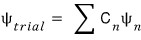
The normalization condition gives $\sum_n|c_n|^2=1$. Now evaluate the Hamiltonian in the trial state:


Using $H\lvert\psi_n\rangle=E_n\lvert\psi_n\rangle$ and orthonormality, all cross terms vanish:
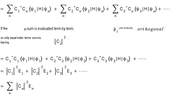
Thus
$$ E_{\mathrm{trial}}=\sum_n |c_n|^2E_n \ge E_0\sum_n|c_n|^2=E_0. $$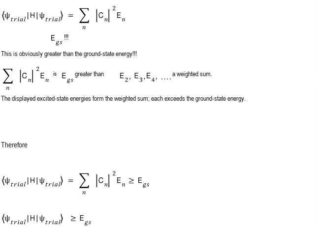
That completes the proof.
Application: the helium ground state
Now let us use the principle on helium, the first atom for which electron–electron repulsion prevents an exact elementary solution.
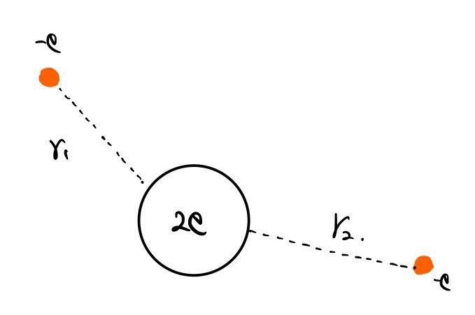
The physical nonrelativistic Hamiltonian is
$$ H=-\frac{\hbar^2}{2m}\left(\nabla_1^2+\nabla_2^2\right) -\frac{e^2}{4\pi\varepsilon_0}\left(\frac{2}{r_1}+\frac{2}{r_2}\right) +\frac{e^2}{4\pi\varepsilon_0r_{12}}, \qquad r_{12}=|\mathbf r_1-\mathbf r_2|. $$
Source correction. The retained source image above places $1/r_{12}$ inside the same overall negative bracket as the nuclear-attraction terms, which would make the electron–electron interaction attractive. It also appears to repeat $\nabla_1^2$ where the second term should be $\nabla_2^2$. The native equation written immediately above is the corrected helium Hamiltonian; the archived image is preserved rather than silently altered.
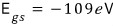
If we ignore electron–electron repulsion, each electron occupies a hydrogenic $1s$ orbital with nuclear charge $+2e$, giving
The measured ground-state energy is approximately
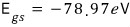
The independent-electron value is far too negative because it neglects the electrons’ mutual repulsion.
A screened-charge trial state
To use the variational method, we first need

A natural first guess is a product of two hydrogenic $1s$ orbitals,

initially with nuclear charge $Z=2$:
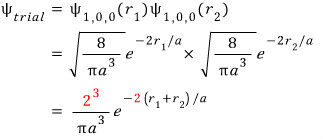
But each electron partially screens the nucleus from the other electron.
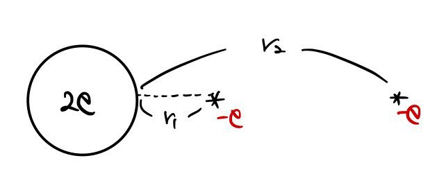
The outer electron therefore feels a weaker attraction than the unscreened term

would suggest. We account for screening by replacing the fixed charge 2 in the orbital with a variational parameter $Z$:
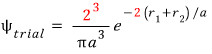
where $a$ is the Bohr radius.
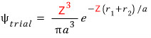
The variational theorem says

so we minimize

with respect to $Z$.
For the calculation, split the correct Hamiltonian into a hydrogenic part with charge $Z$ plus a correction. The retained source first writes

and then rearranges it as

Source correction. As in the earlier Hamiltonian image, the standalone source image at
eq_107.jpgshows the wrong sign for electron–electron repulsion and repeats the first Laplacian. The color-codedeq_111.jpgdecomposition does contain the intended positive $1/r_{12}$ correction, but its red reference Hamiltonian also repeats $\nabla_1^2$ where the second kinetic term should be $\nabla_2^2$. The calculation below uses the physical Hamiltonian written in native math above.
Let $E_1=-13.6\,\mathrm{eV}$ denote the hydrogen ground-state energy.

The two charge-$Z$ one-electron pieces contribute $2Z^2E_1$:

The remaining expectation values give

For a hydrogenic $1s$ orbital,

and the electron–electron repulsion integral is
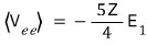
where the expression is positive because $E_1\lt0$. Combining the terms,
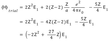
or
$$ E_{\mathrm{trial}}(Z)=\left(-2Z^2+\frac{27}{4}Z\right)E_1. $$Setting $dE_{\mathrm{trial}}/dZ=0$ gives $Z=27/16=1.6875$ and
$$ E_{\mathrm{trial,min}}=\frac{729}{128}E_1 =-\frac{729}{128}(13.6\,\mathrm{eV})\approx-77.5\,\mathrm{eV}. $$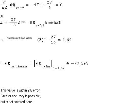
This is within about 2% of the measured value and, as required, lies above it. The source image evaluates the final expression with a rounded label $Z=1.67$; the stationary value is exactly $27/16=1.6875$.
Example 1: harmonic oscillator with a Gaussian trial state
The one-dimensional harmonic-oscillator potential is parabolic:
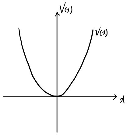
That shape suggests a Gaussian trial function,
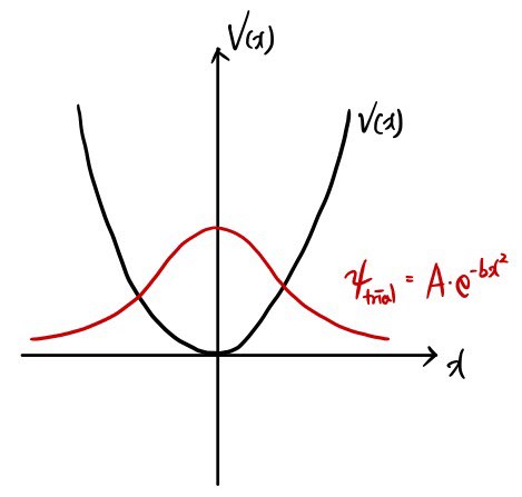

Take
$$ \psi_{\mathrm{trial}}(x)=A e^{-bx^2},\qquad b>0. $$
Normalization requires $\langle\psi_{\mathrm{trial}}|\psi_{\mathrm{trial}}\rangle=1$.
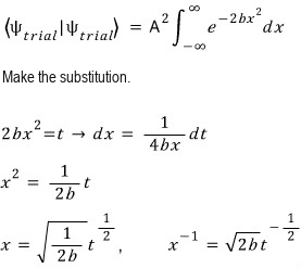
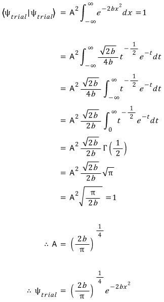
$$ 1=2A^2\int_0^\infty e^{-2bx^2}\,dx =\frac{A^2}{\sqrt{2b}}\int_0^\infty t^{-1/2}e^{-t}\,dt =A^2\sqrt{\frac{\pi}{2b}}. $$Source correction. In
eq_148-en.png, the substitution $t=2bx^2$ is applied to the full interval $-\infty\lt x\lt\infty$ without separating the two branches of $x=\pm\sqrt{t/(2b)}$. The retainedeq_149.jpgthen writes a $t^{-1/2}e^{-t}$ integral over negative $t$, although $t\ge0$. The final constant is correct, but those intermediate limits are not. The valid symmetry-reduced derivation is shown below.
Thus $A=(2b/\pi)^{1/4}$.
With
$$ H=-\frac{\hbar^2}{2m}\frac{d^2}{dx^2}+\frac12m\omega^2x^2, $$we calculate the kinetic and potential contributions separately.
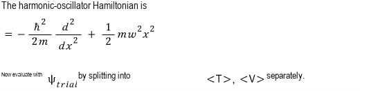
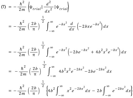
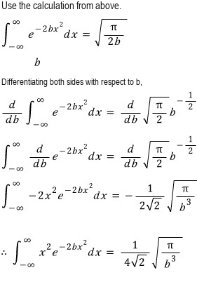
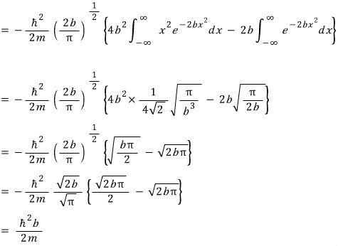
The kinetic term reduces to
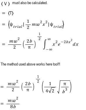
The potential term is
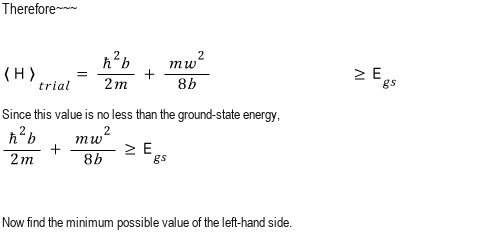
Therefore
and minimization gives
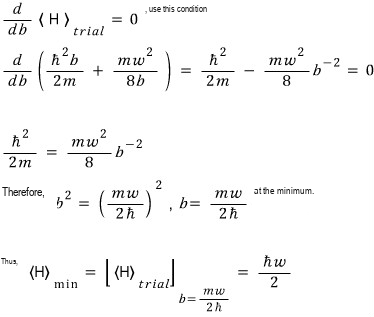
At the minimizing value, $\langle T\rangle=\langle V\rangle=\hbar\omega/4$.
Source correction. The original prose says the energy becomes a maximum when $\langle T\rangle=\langle V\rangle$; it is the minimum of this variational family. The retained
eq_156-en.pngalso states $\langle V\rangle=\langle T\rangle$ before optimization, but the equality holds only at $b=m\omega/(2\hbar)$.
Why did the estimate reproduce the exact answer? We happened to choose the exact functional form:

matches the true ground-state eigenfunction

when $b=m\omega/(2\hbar)$. A poorly chosen family—for example, something much too sharply localized—would yield a higher variational energy.

Problem 7.11: a compact-support cosine trial state
Use

for the one-dimensional harmonic oscillator and optimize $a$. In native form,
$$ \psi_{\mathrm{trial}}(x)= \begin{cases} A\cos(\pi x/a),& |x|\lt a/2,\\ 0,&\text{otherwise}. \end{cases} $$First normalize the state.

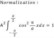
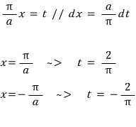
$$ 1=A^2\frac{a}{\pi}\int_{-\pi/2}^{\pi/2}\cos^2t\,dt =A^2\frac{a}{2}. $$Source correction. The endpoint lines in
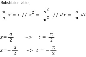
eq_179.jpgare dimensionally and algebraically inconsistent. For $t=\pi x/a$, the actual limits are $x=-a/2\mapsto t=-\pi/2$ and $x=+a/2\mapsto t=+\pi/2$. The corrected normalization is
This gives the correctly normalized result shown next.
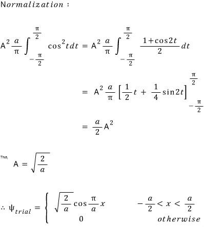
Thus $A=\sqrt{2/a}$.

The kinetic contribution is
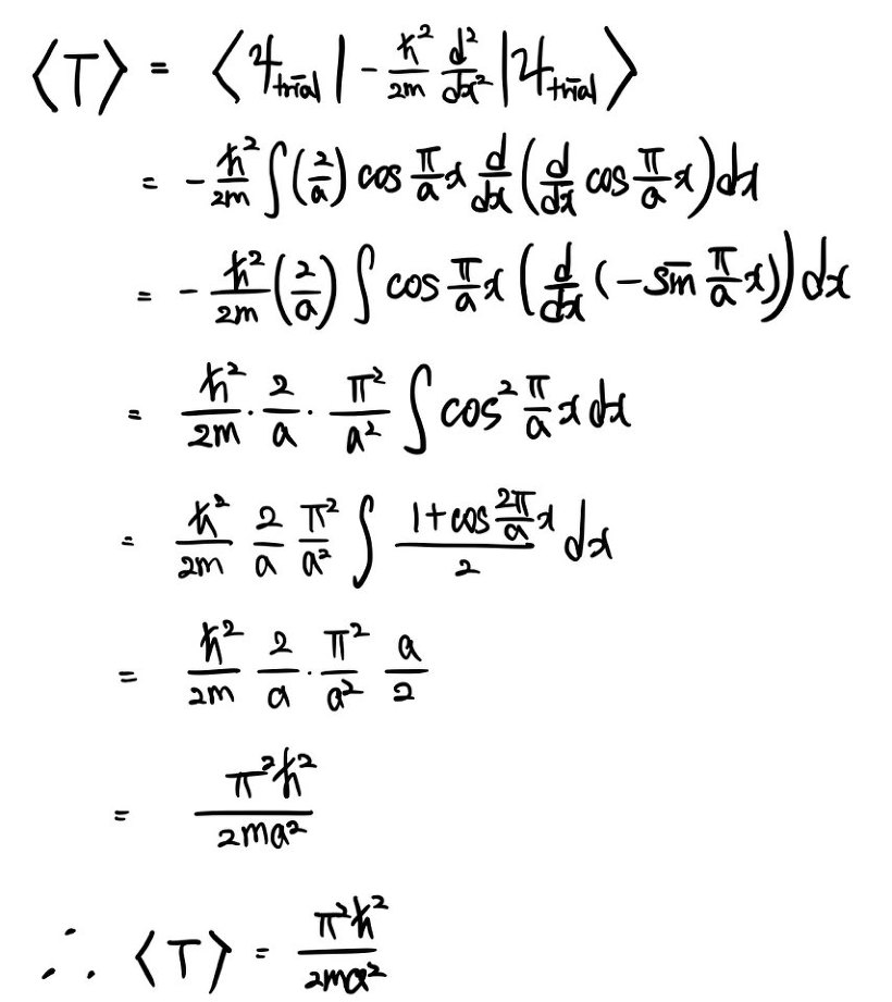
This continuous piecewise cosine belongs to the oscillator’s quadratic-form domain because its weak first derivative is square-integrable. Its first derivative jumps at $x=\pm a/2$, however, so it is generally not in the $H^2$ operator domain of the differential Hamiltonian. The retained img_185.jpg differentiates only on the interior of the support and omits that boundary qualification; the authoritative kinetic value above is the quadratic-form evaluation, not an unqualified application of the pointwise second derivative across the endpoints.
The original post switched to a handwritten photo here—the equation editor was making the calculation more painful than the physics. Fair enough; the derivation is preserved above.
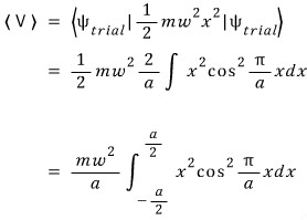
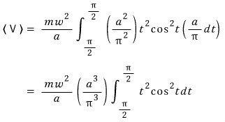
For the potential contribution,
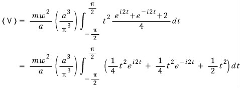
The integration-by-parts identity used is

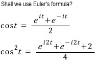
and the detailed evaluation is shown here:
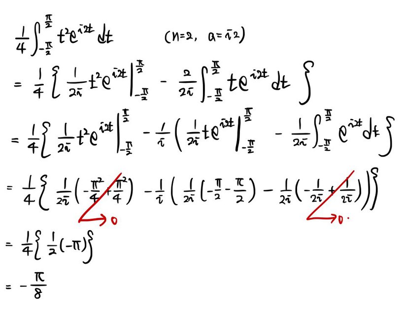
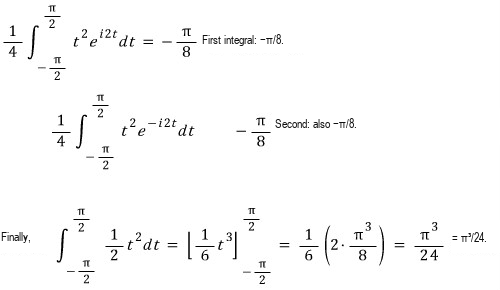
Combining them gives
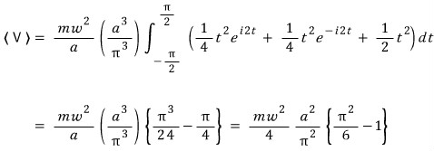
and therefore

Setting $dE_{\mathrm{trial}}/da=0$ yields
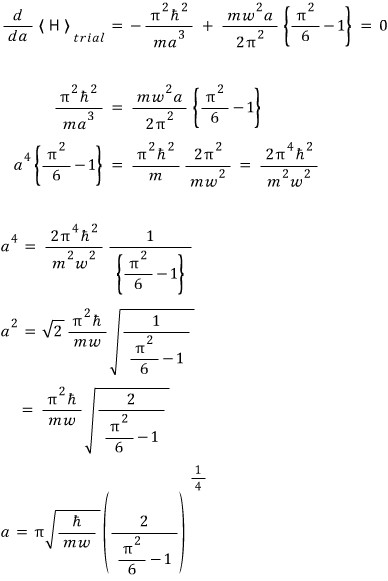
and substitution gives
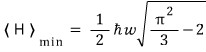

That is,
$$ E_{\mathrm{trial,min}}=\frac12\hbar\omega \sqrt{\frac{\pi^2}{3}-2} \approx0.5679\hbar\omega. $$The exact value is $E_0=0.5\hbar\omega$, so the trial result is higher by $0.0679\hbar\omega$, or about 13.6% relative to the exact energy. The source prose’s “difference of about 0.1357” refers to the excess of the dimensionless square-root factor above 1, not the energy difference itself.
The lesson is exactly what the variational principle promises: the bound is reliable, but its accuracy depends on the trial family.
Problem 7.13: a Gaussian trial state for hydrogen
Now approximate the hydrogen ground state with the Gaussian
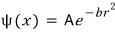
$$ \psi_{\mathrm{trial}}(r)=Ae^{-br^2},\qquad b>0. $$Source notation note. The retained
eq_217.jpglabels the radial Gaussian as $\psi(x)$ even though its exponent uses $r^2$. The radial coordinate is $r$, so the authoritative notation below is $\psi_{\mathrm{trial}}(r)$.
The task is to minimize the upper bound on the ground-state energy. The source problem calls this a “maximum lower bound,” but the variational theorem supplies an upper bound, and minimizing it produces the tightest value within this family.
Normalization begins with
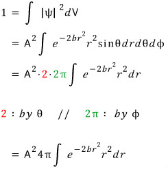
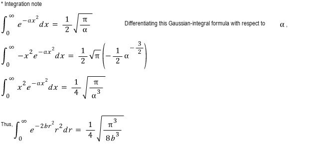
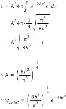
so $A=(8b^3/\pi^3)^{1/4}$.
The hydrogen Hamiltonian is

and the kinetic expectation starts as
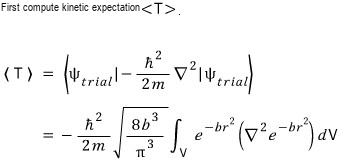
For a spherically symmetric function, only the radial part of the Laplacian contributes:
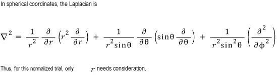
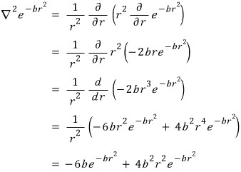
Substitution into the expectation value gives
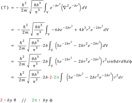
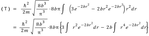

and hence
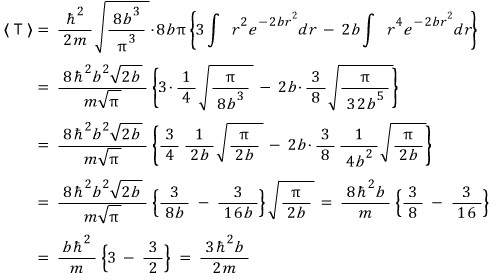
For the Coulomb potential,
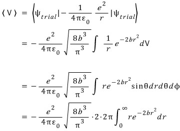
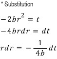
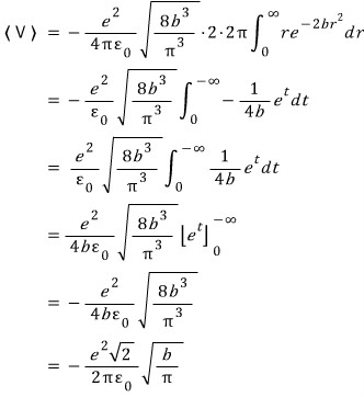
so

Minimizing with respect to $b$ gives
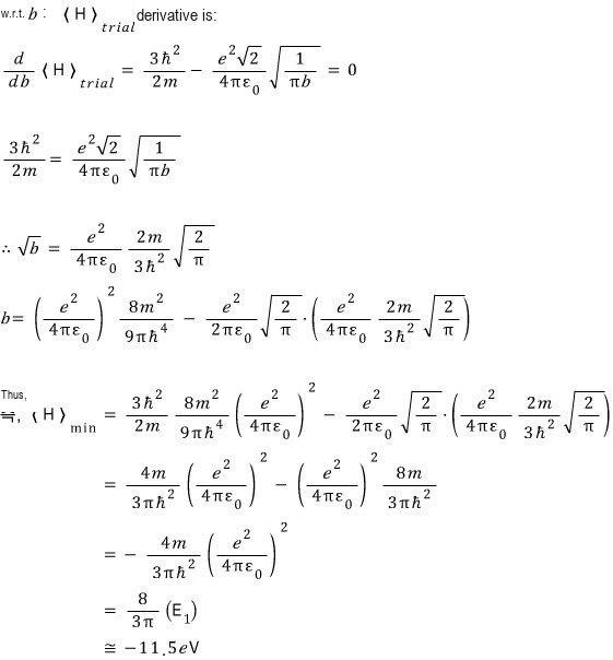
where
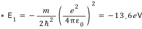
Because $-11.5\,\mathrm{eV}>-13.6\,\mathrm{eV}$, the result obeys the variational bound. Its error is about $2.056\,\mathrm{eV}$, or 15.117% relative to the magnitude of the exact ground-state energy. A Gaussian falls off as $e^{-br^2}$ rather than the exact hydrogenic $e^{-r/a}$, so some error is unavoidable within this one-parameter family.
That is the central habit of variational work: choose a physically sensible family, normalize it, calculate $\langle H\rangle$, and minimize. The theorem guarantees the direction of the error; the quality of the guess determines its size.
Comments
Discussion happens via GitHub Discussions. You'll need a GitHub account to comment.