The WKB Approximation (Wentzel–Kramers–Brillouin)

Alright, Chapter 8 — the WKB approximation.

It’s another one of those “we can’t actually solve the Schrödinger equation exactly, so let’s approximate” methods.

Quick recap of the last two chapters before we dive in.

Ch.6, perturbation theory: use it when there’s a teeeeny tiny little perturbation on top of something you already know.

Ch.7, the variational principle: use it when you have zero intuition for the wave function, so you just guess something and estimate from there. YOLO style.

So when do we reach for Ch.8 — WKB?

1. When $V(x)$ is not constant,
2. But $V(x)$ changes slowly (compared to the wavelength $\lambda$ of the wave function).

In situations like that, WKB is supposedly a good approximation.

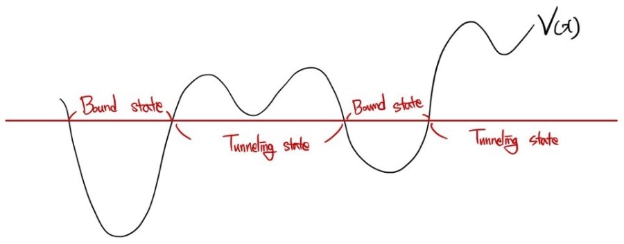
And the nice part: with this one method we can handle both the bound state and the tunneling state~!

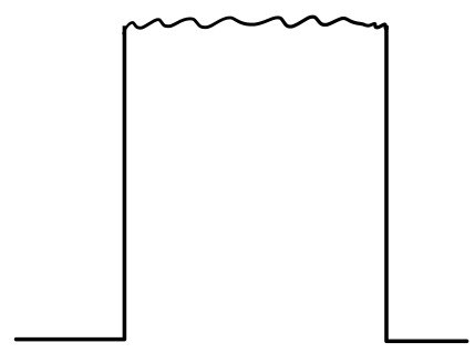
We saw these guys all the way back in Ch.2, so I’ll just throw a quick picture in here.

OK OK OK OK, let’s start with the $V = 0$ case.

I’ll knock out the time-independent equation in 3 seconds.

$$\frac {d^{2}\psi}{dx^{2}}\quad =\quad -\frac {2mE}{\hbar^{2}}\psi \\ k\quad \equiv \quad \sqrt {\frac {2mE}{\hbar^{2}}} \\ \frac {d^{2}\psi}{dx^{2}}\quad =\quad -k^{2}\psi$$$$\text{Differentiated twice, and it's a constant multiple of itself?}\\ \text{Hey now!!! This is!!!}\\ general\quad solution\quad :\\ \psi (x)\quad =\quad Ae^{ikx}\quad +\quad Be^{-ikx}$$

Boom. That’s the general solution for $V = 0$.

Now,

inside a (finite) potential well like this,

$$\psi (x)\quad =\quad Ae^{ikx}\quad +\quad Be^{-ikx}$$

And if $V$ isn’t zero but is just some constant $V$,

$$\psi (x)\quad =\quad Ae^{i\sqrt {2m\left( E-V \right) /\hbar}\cdot x}\quad +\quad Be^{-i\sqrt {2m\left( E-V \right) /\hbar}\cdot x}\\ \quad =\quad Ae^{\pm i\sqrt {2m\left( E-V \right) /\hbar}\cdot x}\quad =\quad Ae^{\pm ikx}$$

that works, right?????? (Yep. It works.)

OK, so where does WKB actually earn its keep?

A situation like this.

Alright~!

Here comes the big WKB assumption.

“In a case like this, the wave function should look like”

$$\psi (x)\quad =\quad A(x)e^{\pm ik(x)\cdot x}$$

The amplitude now depends on position. Not totally crazy, right?

(Note: $k(x)$ being position-dependent is the obvious part — of course it is. The real assumption here is that the amplitude $A$ is position-dependent too.

Why $k(x)$ being a function of $x$ is natural will become clear in a sec.)

From here we’ll split into two cases — bound state, then tunneling state — and handle them one at a time.

Let’s go in first!!!!! The classical region!!

Huh? What’s the classical region? That’s the bound state.

Because $E > V$ is the case that makes intuitive sense (and classical sense).

(The one that doesn’t make intuitive sense is $E < V$, the tunneling state. That one’s called the non-classical region!)

OK let me write the time-independent Schrödinger equation again for the bound state.

$$-\frac {\hbar^{2}}{2m}\frac {d^{2}}{dx^{2}}\psi \quad +\quad V(x)\psi \quad =\quad E\psi \\ \text{Let the games begin.} \\ -\frac {\hbar^{2}}{2m}\frac {d^{2}}{dx^{2}}\psi \quad =\quad \left( E\quad -\quad V(x) \right) \psi \\ \frac {d^{2}\psi}{dx^{2}}\quad =-\frac {2m}{\hbar^{2}}\left( E\quad -\quad V(x) \right) \psi \quad \\ =\quad -\frac {\left( \sqrt {2m(E-V(x))} \right)^{2}}{\hbar^{2}}\psi \\ \text{That red guy there,} \\ \text{'the momentum a particle of energy } E \text{ and mass } m \text{ has passing through a region of potential } V(x)\text{'}\\ \text{we can read it that way, right??!??! } \\ \text{So,} \\ \frac {d^{2}\psi}{dx^{2}}\quad =\quad -\frac {\left( \sqrt {2m(E-V(x))} \right)^{2}}{\hbar^{2}}\psi \quad \\ \quad =\quad -\frac {p(x)^{2}}{\hbar^{2}}\psi$$

(Now do you see why $k(x)$ being a function of $x$ is natural???)

Anyway — time for the grand operation of expressing $k(x)$ and $A(x)$ in terms of $p$.

Back in the finite potential well, momentum was a constant. Now $p$ is a function of $x$!

Let’s grab the wave function we assumed,

$$\psi (x)\quad =\quad A(x)e^{\pm ik(x)\cdot x}$$

and put it to work.

We need the second derivative of

$$\psi (x)$$

but differentiating $k(x)\cdot x$ is messy, so let’s set

$$k(x)\cdot x\quad \equiv \quad \varphi (x)$$

and go from there.

$$\frac {d}{dx}\psi (x)\quad =\quad \frac {d}{dx}\left( A(x)e^{i\varphi (x)} \right) \quad \\ =\quad A'(x)e^{i\varphi (x)}\quad +\quad A(x)i\varphi '(x)e^{i\varphi (x)}\\ \quad =\left\{A'(x)\quad +\quad iA(x)\varphi '(x) \right\} e^{i\varphi (x)}$$$$\text{One more time~}\\ \frac {d^{2}\psi}{dx^{2}}\quad =\quad \frac {d}{dx}\left( \left\{A'(x)\quad +\quad iA(x)\varphi '(x) \right\} e^{i\varphi (x)} \right) \quad \\ \\ =\quad \left( A'(x)+iA(x)\varphi '(x) \right) 'e^{i\varphi (x)}\quad +\quad i\varphi '(x)\left( A'(x)\quad +\quad iA(x)\varphi '(x) \right) e^{i\varphi (x)}\\ =\quad \left( A''(x)\quad +\quad iA'(x)\varphi '(x)\quad +\quad iA(x)\varphi ''(x) \right) e^{i\varphi (x)}\quad +\quad \left( -A(x)\varphi '(x)^{2}+\quad iA'(x)\varphi '(x) \right) e^{i\varphi (x)}\\ =\quad \left\{\left( A''(x) \right) \quad -\quad A(x)\varphi '(x)^{2}\quad +\quad i\left( 2A'(x)\varphi '(x)\quad +A(x)\varphi ''(x) \right) \right\} e^{i\varphi (x)}$$

Now let’s write

$$\frac {d^{2}\psi}{dx^{2}}\quad =\quad -\frac {p(x)^{2}}{\hbar^{2}}\psi$$

again.

On the left we stick in what we just computed, on the right we sub in

$$\psi (x)\quad =\quad A(x)e^{i\varphi (x)}$$

~

$$\left\{\left( A''(x) \right) \quad -\quad A(x)\varphi '(x)^{2}\quad +\quad i\left( 2A'(x)\varphi '(x)\quad +A(x)\varphi ''(x) \right) \right\} e^{i\varphi (x)}\quad =\quad -\frac {p(x)^{2}}{\hbar^{2}}A(x)e^{i\varphi (x)}$$

The $e^{i\varphi(x)}$ cancels on both sides, and we split into real and imaginary parts.

$$Real\quad :\quad A''(x)\quad -A(x)\Phi '(x)^{2}\quad =\quad -\frac {p(x)^{2}}{\hbar^{2}}A(x)\\ \quad \\ \quad \to \quad A''(x)\quad =\quad A(x)\left( \varphi '(x)^{2}\quad -\quad \frac {p(x)^{2}}{\hbar^{2}} \right)$$$$Imaginary\quad :\quad 2A'(x)\varphi '(x)\quad +\quad A(x)\varphi ''(x)\quad =\quad 0 \\ \to \quad \frac {\left( A^{2}(x)\varphi '(x) \right) '}{A(x)}=0\\ \quad \\ \therefore \quad A^{2}(x)\varphi '(x)\quad \text{is constant}$$

​Let’s pause and package up what we have so far.

$$\text{Call the constant value of } A^{2}(x)\varphi '(x)\text{, from the imaginary part, }C'^{2}\text{.}\\ A^{2}(x)\varphi '(x)\quad =\quad C'^{2}\\ A^{2}(x)\quad =\quad \frac {C'^{2}}{\varphi '(x)}\\ A(x)\quad =\quad \frac {C'}{\sqrt {\varphi '(x)}}$$

I deliberately wrote it as a square. On purpose.

Why the prime on it though… heh.

That’ll be revealed in about 60 seconds.

Before that, let me draw a conclusion from the equation above.

$$\psi (x)\quad =\quad A(x)e^{i\varphi (x)}\quad =\quad \frac {C'}{\sqrt {\varphi '(x)}}e^{i\varphi (x)}$$

Ahhh~~~~ $A(x)$ is determined!!!! Well — determined as soon as we know $\varphi'(x)$.

There should be a hint in the real-part equation!

$$Real\quad :\quad A''(x)\quad -A(x)\Phi '(x)^{2}\quad =\quad -\frac {p(x)^{2}}{\hbar^{2}}A(x)\\ \quad \\ \quad \to \quad A''(x)\quad =\quad A(x)\left( \varphi '(x)^{2}\quad -\quad \frac {p(x)^{2}}{\hbar^{2}} \right)$$

From here, we’re going to set

$$A''(x)\quad =\quad 0$$

Why? Because the whole point was: $A(x)$ changes slowly.

In a finite-potential-well setup where $V$ changes just a tiny bit at a time, we expect $A$ to change so gently that it has no inflection point.

So the real-part equation becomes

$$A''(x)\quad =\quad A(x)\left( \varphi '(x)^{2}\quad -\quad \frac {p(x)^{2}}{\hbar^{2}} \right) \quad =\quad 0 \\ \therefore \quad \varphi '(x)^{2}\quad =\quad \frac {p(x)^{2}}{\hbar^{2}}\\ \varphi '(x)\quad =\quad \frac {d\varphi (x)}{dx}\quad =\quad \pm \sqrt {\frac {p(x)}{\hbar}} \\ \varphi (x)\quad =\quad \pm \int {\sqrt {\frac {p(x)}{\hbar}}}dx$$

and we can write it like that.

Now $A(x)$ is fully determined too!!!! Plug back into the imaginary-part conclusion,

$$\psi (x)\quad =\quad \frac {C'}{\sqrt {\varphi '(x)}}e^{i\varphi (x)}\quad \\ =\quad \frac {C'}{\sqrt {\left| \frac {p(x)}{\hbar} \right|}}e^{\pm i\int {\frac {p(x)}{\hbar}}dx}\quad \\ =\quad \frac {C'\hbar}{\sqrt {\left| p(x) \right|}}e^{\pm \frac {i}{\hbar}\int {p(x)}dx}\quad \equiv \frac {C}{\sqrt {\left| p(x) \right|}}e^{\pm \frac {i}{\hbar}\int {p(x)}dx}\\ \quad \psi (x)\quad =\quad \frac {C}{\sqrt {\left| p(x) \right|}}e^{\pm \frac {i}{\hbar}\int {p(x)}dx}$$

WE GOT THE WAVE FUNCTION IN THE CLASSICAL REGION!!!!!!!!!!!!! (via WKB.)

​

$$\psi (x)\quad =\quad \frac {C}{\sqrt {\left| p(x) \right|}}e^{i\varphi (x)}$$

​And this isn’t even that unphysical! It actually checks out.

Because the probability-of-finding-the-particle — the mod-squared —

$$\left| \psi (x) \right|^{2}\quad \propto \quad \frac {1}{p(x)}~\frac {1}{v}$$

so when $v$ gets large, the probability drops,

and when $v$ gets small, the probability rises —

which… makes sense, right? Fast particle, less time in any one spot, less likely to be found there. That’s why I said it’s not unphysical.

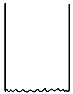
OK, let’s do an example and a problem for the classical region.

Consider something like this (an infinite potential well).

If we apply the WKB approximation,

$$\psi (x)\quad =\quad \frac {C}{\sqrt {\left| p(x) \right|}}e^{\pm \frac {i}{\hbar}\int {p(x)}dx}$$

inside the well both right-going and left-going waves coexist, so

$$\psi (x)\quad =\quad \frac {1}{\sqrt {\left| p(x) \right|}}\left( C_{1}e^{\frac {i}{\hbar}\int {p(x)}dx}\quad +\quad C_{2}e^{-\frac {i}{\hbar}\int {p(x)}dx} \right)$$

write it like that!!!!

And let’s define

$$\frac {1}{\hbar}\int {p(x)}dx\quad \equiv \quad \varphi (x)$$

so it’s cleaner!!

$$\psi (x)\quad =\quad \frac {1}{\sqrt {\left| p(x) \right|}}\left( C_{1}e^{i\varphi (x)}\quad +\quad C_{2}e^{-i\varphi (x)} \right)$$

Now write it like this!!!!!!

Because we want trig functions!!!

$$\psi (x)\quad =\quad \frac {1}{\sqrt {\left| p(x) \right|}}\left( C_{1}\left( cos\varphi (x)\quad +\quad isin\Phi (x) \right) \quad +\quad C_{2}\left( cos\varphi (x)\quad -\quad isin\Phi (x) \right) \right) \\ \quad =\frac {1}{\sqrt {\left| p(x) \right|}}\left( \left( C_{1}+C_{2} \right) cos\varphi (x)\quad +i\left( C_{1}-C_{2} \right) sin\Phi (x) \right) \\ \quad =\frac {1}{\sqrt {\left| p(x) \right|}}\left( C_{1}'cos\varphi (x)\quad +iC_{2}'sin\Phi (x) \right)$$

There — that’s our wave function!!!! Now boundary conditions.

$$\text{B.C.} \quad :\quad \psi (0)\quad =\quad \psi (a)\quad =\quad 0$$$$\psi (0)\quad =\quad \frac {1}{\sqrt {\left| p(0) \right|}}\left( C_{1}'cos\varphi (0)\quad +iC_{2}'sin\Phi (0) \right) \\ \text{Since }\varphi (x)\quad =\quad \frac {1}{\hbar}\int _{0}^{x}{p(x')dx'}\text{, we have }\varphi (0)\quad =\quad 0\text{.} \\ \text{So }\varphi (0)\quad =\quad \frac {1}{\sqrt {\left| p(0) \right|}}\left( C_{1}' \right) \quad =\quad 0\\ \text{Which gives }C_{1}'\quad =\quad 0\text{. Update the wave function.}$$$$\psi (x)\quad =\frac {1}{\sqrt {\left| p(x) \right|}}iC_{2}'sin\Phi (x)\\ \text{Second B.C.}\\ \psi (a)\quad =\frac {1}{\sqrt {\left| p(a) \right|}}iC_{2}'sin\Phi (a)\quad =\quad 0 \\ \text{So we need }\Phi (a)\quad =\quad n\pi \\ \text{That is, }\frac {1}{\hbar}\int _{0}^{a}{p(x)dx}\quad =\quad n\pi \\ \int _{0}^{a}{p(x)dx}\quad =\quad n\pi \hbar$$

Since

$$p(x)\quad =\quad \sqrt {2m(E-V(x)}$$

if $V(x)$ is some bumpy thing, there’s nothing more we can do.

So… let’s at least sanity-check this formula.

Plug in $V(x) = 0$. It had better reduce to the usual infinite-well energies.

$$\text{If }V(x)\quad =\quad 0\text{, then }p(x)\quad =\quad \sqrt {2mE} \\ \text{So }\int _{0}^{a}{p(x)dx}\quad =\quad n\pi \hbar \\ \int _{0}^{a}{\sqrt {2mE}dx}\quad =\quad n\pi \hbar \\ =\quad a\sqrt {2mE} \\ a^{2}2mE\quad =\quad n^{2}\pi^{2}\hbar^{2}\\ E_{n}\quad =\quad \frac {n^{2}\pi^{2}\hbar^{2}}{2ma^{2}}$$

Ahhh, the proper infinite-well energies fall right out.

Good good good — we’ve (somewhat forcibly) convinced ourselves that WKB isn’t lying.

Tunneling state

Now — the region that makes no sense. The tunneling state!!!!

The non-physical region, so named because, well, it makes no physical sense!!!

We hit cases like this back in Ch.2.

Back then we did tunneling by flipping the finite-well setup upside down.

Now, since WKB is for when $V$ changes slowly,

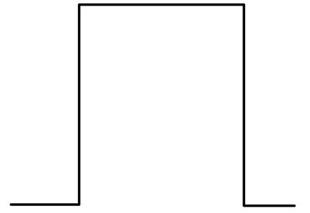
what kind of setup are we actually looking at here?

Something like this!?

Let’s just hold that picture loosely for now, and when we get to the problems later, we’ll see exactly what kind of situation calls for WKB in the tunneling region!!

Here’s the kicker — deriving the wave function in the tunneling state is exaaactly the same as deriving it in the bound state we just did.​

​

​

The only difference is $E > V$ vs. $E < V$.

So now

$$p(x)\quad =\quad \sqrt {2m(E-V(x))}$$

this guy goes imaginary… T_T

Because the thing under the square root is negative now!!!!! So

$$p(x)\quad =\quad i\sqrt {2m(E-V(x))}$$

is how it has to be written!!! And that’s the only change — everything else is the same!

$$\psi (x)\quad =\quad \frac {C}{\sqrt {\left| p(x) \right|}}e^{\pm \frac {i}{\hbar}\int {p(x)}dx}$$

Rewrite with the new $p$!

$$\psi (x)\quad =\quad \frac {C}{\sqrt {\left| p(x) \right|}}e^{\mp \frac {1}{\hbar}\int {p(x)}dx}$$

Done!!!!!!!!!! Tunneling-state wave function — done!!!!

(The constant out front was already inside an absolute value, so I didn’t touch it!! We’re good, right?!)

That was almost suspiciously fast.

OK let’s go ahead and

describe the bound and tunneling states together.

(Because, like — observing tunneling all by itself isn’t really a thing. It only makes sense hooked up to the bound region on either side.)

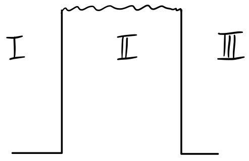
Let’s put a picture like this into equations!!!!!!

(Same logic as Ch.2.)

Region Ⅰ

$$\psi (x)\quad =\quad Ae^{ikx}\quad +\quad Be^{ikx}\quad \text{Do we even need WKB here~? It's flat.}\approx ~~?$$

Region Ⅱ

$$\psi (x)\quad =\quad \frac {C}{\sqrt {\left| p(x) \right|}}e^{\frac {1}{\hbar}\int {\left| p(x) \right| dx}}\quad -\quad \frac {D}{\sqrt {\left| p(x) \right|}}e^{-\frac {1}{\hbar}\int {\left| p(x) \right| dx}}$$

Region Ⅲ

$$\psi (x)\quad =\quad Fe^{ikx}$$

The red one’s the growing piece, the blue one’s the decaying piece!!!!

Now the catch:

In Ch.2, $V$ was constant, so we could pin down all the constants.

Here we can’t.

But we’re not totally stuck.

Same as in Ch.2 — the point was never to find the tunneling wave function itself.

The point was the transmission coefficient $T$.

$$\text{Transmission coefficient}\quad :\quad T\quad =\quad \frac {\text{amplitude of transmitted wave}}{\text{amplitude of incident wave}}\quad =\quad \frac {F}{A}$$

Getting this (useful in the lab, btw) was the actual goal.

And intuitively —

doesn’t $T$ basically live or die on the decaying factor

$$e^{-\frac {1}{\hbar}\int {\left| p(x) \right| dx}}$$

?!

That is, the transmission coefficient

$$\text{transmission coefficient}\quad =\quad \frac {\left| F \right|^{2}}{\left| A \right|^{2}}$$

should go like

$$e^{-\frac {2}{\hbar}\int {\left| p(x) \right| dx}}$$

!!!!

At least that’s what we’re guessing… T_T hahahahahaha

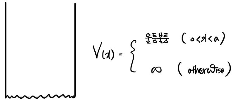
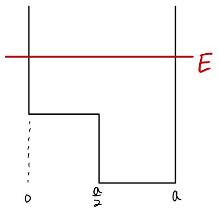
Prob 8.1

Using the WKB approximation, find the allowed energies $E_n$ for an infinitely deep square well where half of the well has a “shelf” at height $V_0$.

First: writing $\psi(x)$ with WKB, the derivation is identical to the bound-state walkthrough above, right up to

$$\psi (x)\quad =\quad \frac {1}{\sqrt {p(x)}}\left\{C_{1}'cos\varphi (x)\quad +\quad C_{2}'sin\Phi (x) \right\}$$

And in this problem too!!! since $V = \infty$ at $x = 0$ and $x = a$,

$$\psi (0)\quad =\quad \psi (a)\quad =\quad 0$$

So,

$$\text{From }\psi (0)\quad =\quad 0\text{ we get }C_{1}'\quad =\quad 0\text{,}\\ \text{from }\psi (a)\quad =\quad 0\text{ we get }\varphi (a)\quad =\quad n\pi\text{, and from that}\\ \frac {1}{\hbar}\int _{0}^{a}{p(x)dx}\quad =\quad n\pi \quad \text{.}$$

And now — unlike before, where $V(x)$ was just “bumpy” and we were stuck — $V(x)$ has an actual formula.

So the integral is doable. Let’s crunch it.

$$n\pi \hbar \quad =\quad \int _{0}^{a}{p(x)}dx\quad \\ =\quad \int _{0}^{a}{\quad}\sqrt {2m(E-V(x)}dx\quad \\ =\quad \int _{0}^{\frac {a}{2}}{\quad}\sqrt {2m(E-V_{0})}dx\quad +\quad \int _{\frac {a}{2}}^{a}{\quad}\sqrt {2mE}dx\\ =\quad \frac {a}{2}\sqrt {2m(E-V_{0})}\quad +\quad \frac {a}{2}\sqrt {2mE}\quad =\quad n\pi \hbar \\ \\ \frac {a}{2}\sqrt {2m}\left( \sqrt {E-V_{0}}\quad +\quad \sqrt {E}\quad \right) \quad =\quad n\pi \hbar \quad \text{square both sides, here we go}\\ \frac {a^{2}}{4}2m\left( E-V_{0}+E+2\sqrt {E\left( E-V_{0} \right)} \right) \quad =\quad n^{2}\pi^{2}\hbar^{2}\\ 2E-V_{0}+2\sqrt {E\left( E-V_{0} \right)}\quad =\quad 4\frac {n^{2}\pi^{2}\hbar^{2}}{2ma^{2}}\quad =\quad 4E_{n} \\ 2\sqrt {E\left( E-V_{0} \right)}\quad =\quad \left( 4E_{n}+V_{0}-2E \right) \quad \text{square both sides again, here we go} \\ 4E^{2}-4EV_{0}\quad =\quad 16E_{n}^{2}\quad +\quad 4E^{2}\quad +\quad V_{0}^{2}\quad -\quad 16E\cdot E_{n}\quad +\quad 8E_{n}V_{0}\quad -\quad 4EV_{0} \\ 16E\cdot E_{n}\quad =\quad 16E_{n}^{2}\quad +\quad V_{0}^{2}\quad +\quad 8E_{n}V_{0}$$$$\therefore \quad E\quad =\quad E_{n}\quad +\quad \frac {V_{0}^{2}}{16E_{n}}\quad +\quad \frac {V_{0}}{2}$$

Ex. 8.2 — Gamow’s theory of alpha decay

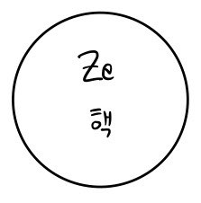
Say we have a nucleus with charge number $Z$ like that.

Inside, the electromagnetic force and the strong force are both at work.

(Strong force between the protons!)

But the larger $Z$ gets, the stronger the proton-proton repulsion. And the nucleus… apparently sometimes shrinks by spitting out its own constituent protons one at a time.

When the thing popping out happens to be a helium ion — that’s an $\alpha$-particle, it’s light,

so boom, alpha radiation!!!

Now let’s draw a potential on top of that picture,

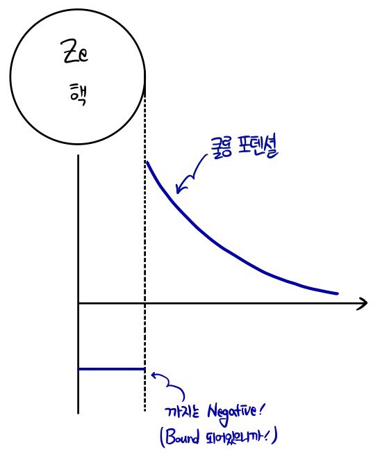
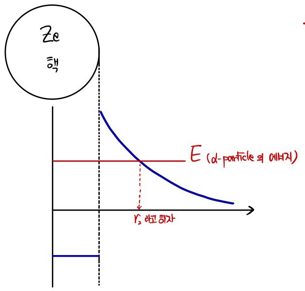
and we can read off what $E$ is from the Coulomb potential.

The Coulomb potential at distance $r_2$ equals $E$, so

$$E\quad =\quad \frac {1}{4\pi \epsilon_{0}}\frac {2Ze^{2}}{r_{2}}$$

OK so now — using the transmission formula we set up earlier,

$$(\text{Transmission coefficient})\quad T\quad \sim\quad e^{-\frac {2}{\hbar}\int _{r_{1}}^{r_{2}}{\sqrt {2m(V(x)-E)}dr}}\quad =\quad e^{-\frac {2}{\hbar}\int _{r_{1}}^{r_{2}}{\sqrt {2m(\frac {1}{4\pi \epsilon_{0}}\frac {2Ze^{2}}{r}-E)}dr}}\\ \\ =\quad e^{-\frac {2}{\hbar}\int _{r_{1}}^{r_{2}}{\sqrt {2m(\frac {1}{4\pi \epsilon_{0}}\frac {2Ze^{2}r_{2}}{rr_{2}}-E)}dr}}\quad \\ =\quad e^{-\frac {2}{\hbar}\int _{r_{1}}^{r_{2}}{\sqrt {2m(E\frac {r_{2}}{r}-E)}dr}}\quad \\ =\quad e^{-\frac {2\sqrt {2mE}}{\hbar}\int _{r_{1}}^{r_{2}}{\sqrt {(\frac {r_{2}}{r}-1)}dr}}$$$$\int _{r_{1}}^{r_{2}}{\sqrt {(\frac {r_{2}}{r}-1)}dr}\quad \text{can apparently be done with the substitution }r=r_{2}sin^{2}u\text{.} \\ dr\quad =\quad 2r_{2}sinucosudu\\ sin^{2}u\quad =\quad \frac {r}{r_{2}}\\ sinu\quad =\quad \sqrt {\frac {r}{r_{2}}}\\ u=sin^{-1}\left( \sqrt {\frac {r}{r_{2}}} \right)$$$$\text{So,}\\ =\quad \int _{sin^{-1}\sqrt {\frac {r_{1}}{r_{2}}}}^{\frac {\pi}{2}}{\quad}\sqrt {\frac {r_{2}}{r_{2}sin^{2}u}\quad -\quad 1}\quad 2r_{2}sinucosu\cdot du\\ =\quad \int _{sin^{-1}\sqrt {\frac {r_{1}}{r_{2}}}}^{\frac {\pi}{2}}{\quad}\frac {\sqrt {1-sin^{2}u}}{sinu}\quad 2r_{2}sinucosu\cdot du\\ =\quad \int _{sin^{-1}\sqrt {\frac {r_{1}}{r_{2}}}}^{\frac {\pi}{2}}{\quad}2r_{2}cos^{2}udu\quad =\quad 2r_{2}\left[ \frac {1}{2}u+\frac {1}{4}sin2u \right]_{sin^{-1}\sqrt {\frac {r_{1}}{r_{2}}}}^{\frac {\pi}{2}}\quad =\quad 2r_{2}\left[ \frac {1}{2}u+\frac {1}{2}sinucosu \right]_{sin^{-1}\sqrt {\frac {r_{1}}{r_{2}}}}^{\frac {\pi}{2}}\\ =\quad 2r_{2}\left[ \frac {1}{2}u+\frac {1}{2}sinu\sqrt {1-sin^{2}u} \right]_{sin^{-1}\sqrt {\frac {r_{1}}{r_{2}}}}^{\frac {\pi}{2}}\quad \\ =\quad 2r_{2}\left[ \left( \frac {1}{2}\frac {\pi}{2}\quad +\quad \frac {1}{2}sin\frac {\pi}{2}\sqrt {1-sin\frac {\pi}{2}} \right) \quad -\quad \left( \frac {1}{2}sin^{-1}\sqrt {\frac {r_{1}}{r_{2}}}\quad +\quad \frac {1}{2}sin\left( sin^{-1}\sqrt {\frac {r_{1}}{r_{2}}} \right) \sqrt {1-\left( sin\left( sin^{-1}\sqrt {\frac {r_{1}}{r_{2}}} \right) \right)^{2}} \right) \right] \\ =\quad 2r_{2}\left\{\frac {\pi}{4}\quad -\quad \frac {1}{2}sin^{-1}\sqrt {\frac {r_{1}}{r_{2}}}\quad -\quad \frac {1}{2}\sqrt {\frac {r_{1}}{r_{2}}}\sqrt {1-\frac {r_{1}}{r_{2}}} \right\} \quad =\quad 2r_{2}\left\{\frac {\pi}{4}\quad -\quad \frac {1}{2}sin^{-1}\sqrt {\frac {r_{1}}{r_{2}}}\quad -\quad \frac {1}{2}\sqrt {\frac {r_{1}}{r_{2}}}\sqrt {\frac {r_{2}-r_{1}}{r_{2}}} \right\} \\ =\quad r_{2}\left\{\frac {\pi}{2}\quad -\quad sin^{-1}\sqrt {\frac {r_{1}}{r_{2}}}\quad -\quad \frac {1}{r_{2}}\sqrt {r_{1}\left( r_{2}-r_{1} \right)} \right\}$$$$T\quad \sim\quad e^{-\frac {2}{\hbar}\sqrt {2mE}\cdot r_{2}\left\{\frac {\pi}{2}\quad -\quad sin^{-1}\sqrt {\frac {r_{1}}{r_{2}}}\quad -\quad \frac {1}{r_{2}}\sqrt {r_{1}\left( r_{2}-r_{1} \right)} \right\}}\\ \quad =\quad e^{-\frac {2}{\hbar}\sqrt {2mE}\left\{r_{2}\left( \frac {\pi}{2}\quad -\quad sin^{-1}\sqrt {\frac {r_{1}}{r_{2}}} \right) \quad -\quad \sqrt {r_{1}\left( r_{2}-r_{1} \right)} \right\}}$$

Now — what do we do with this monster?

Computing $T$ wasn’t really the endgame.

What we actually want is the lifetime of the radioactive element~

Picture an alpha particle bouncing around inside the nucleus at speed $v$.

If it’s trapped inside a sphere of size

$$2r_{1}$$

then the collision frequency (how often it bangs against the wall) is

$$\frac {v}{2r_{1}}$$

It slams into the wall that often per second, and each time the probability of punching through is

$$e^{-2\gamma}$$

apparently.

So the transmission rate per second is

$$\frac {v}{2r_{1}}e^{-2\gamma}$$

And the reciprocal of that… we call the “lifetime of the nucleus.”

$$\text{Parent nucleus's life time}\quad :\quad \tau \quad =\quad \frac {2r_{1}}{v}e^{2\gamma}$$

Take the log,

$$ln\tau \quad =\quad 2\gamma \quad +\quad constant\quad \sim\quad \frac {C_{1}}{\sqrt {E}}\quad +\quad C_{2}$$

and this is the punchline we were after.

$\ln\tau$ is inversely proportional to $\sqrt{E}$!!!!!!

Inversely proportional to energy to the 1/2 power!!!!!!

---

Originally written in Korean on my Naver blog (2015-12). Translated to English for gdpark.blog.