Time-Dependent Perturbation Theory

How does an atom respond when an electric field is switched on? To answer that question, we need to follow its quantum state through time. This post develops the amplitude equations for a two-level system, uses symmetry to evaluate hydrogen dipole matrix elements, and solves an exactly tractable example with constant coupling.

From stationary states to changing populations

In time-independent perturbation theory, we split the Hamiltonian into a solvable part and a small correction:

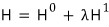
The parameter $\lambda$ keeps track of the perturbation’s order. We use the known eigenstates of $H^0$ to approximate the energies and eigenstates of the full Hamiltonian; the perturbing operator itself is an input to the calculation.

Now allow the perturbation to depend on time:

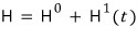
I will denote this perturbation by $H'(t)$ below. An applied electric field is one example. The time-dependent Schrödinger equation still governs the state:

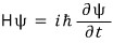
For a time-independent Hamiltonian, an energy eigenstate has a particularly simple time dependence:

Its phase has unit magnitude, so its position probability density $|\psi(x,t)|^2$ is stationary. The probability of finding the particle in a region is the integral of that density over the region. This does not mean that every state of a time-independent Hamiltonian has a stationary density: a superposition of different energies can have time-dependent interference terms.

Expand the initial state in an orthonormal energy eigenbasis:

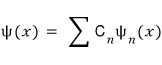
Without a perturbation, each component acquires its own energy-dependent phase:

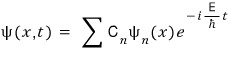
The coefficients $C_n$ are constant in this representation, and the energy-basis probabilities $|C_n|^2$ remain constant. With a perturbation, retain those known phases and let the coefficients vary:

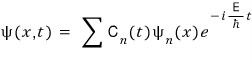
The quantities $C_n(t)$ are probability amplitudes, and $|C_n(t)|^2$ is the population of the corresponding unperturbed basis state. For a nondegenerate level, this is also the probability of measuring its energy with $H^0$. If several basis states share the same energy, add their populations to obtain the probability of that energy. These populations can change when the perturbation couples different states. Explicit time dependence alone does not guarantee population transfer: a perturbation diagonal in this fixed basis can change phases without changing populations.

Factoring out the evolution generated by $H^0$ is the interaction-picture approach. It makes the remaining dynamics easier to isolate. MIT’s time-dependent perturbation theory notes develop this construction in an orthonormal eigenbasis of $H^0$.

This framework will lead us to absorption and stimulated emission, and eventually to the physics behind lasers. Spontaneous emission requires an additional treatment of the atom’s coupling to the quantized radiation field; a prescribed classical field by itself does not explain it.

Deriving the two-level amplitude equations

Start with two unperturbed levels, labeled $a$ and $b$:

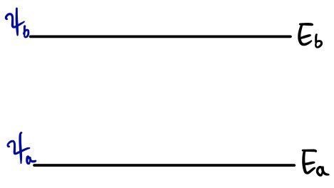
The lower-state spatial wavefunction is

and the upper-state spatial wavefunction is

They are eigenfunctions of $H^0$:

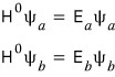
Choose them to be normalized and orthogonal:

Before adding the perturbation, their superposition evolves as follows:

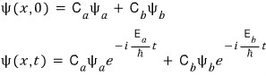
When the perturbation is present, write the state with time-dependent coefficients:

For a genuinely two-dimensional Hilbert space, this expansion is exact. When we use it for an atom with many levels, neglecting the other states is a physical approximation that must be justified.

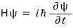
Substitute the expansion into the Schrödinger equation:

First expand the Hamiltonian side, labeled LHS here:

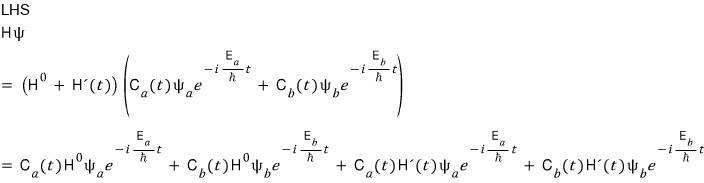
Use the unperturbed eigenvalue equations:

This gives

Next differentiate both the coefficients and the exponential factors on the RHS:

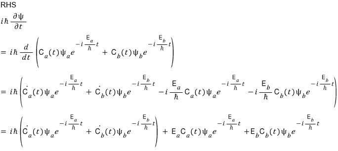
Equate the two expressions:

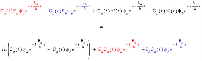
The matching energy terms cancel:

We are left with an equation relating the perturbation to the rates of change of the amplitudes. Project it onto the lower state using

and onto the upper state using

Define the perturbation matrix elements by

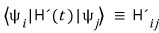
The first index labels the bra and the second labels the ket. Orthonormality then gives one equation for each coefficient:

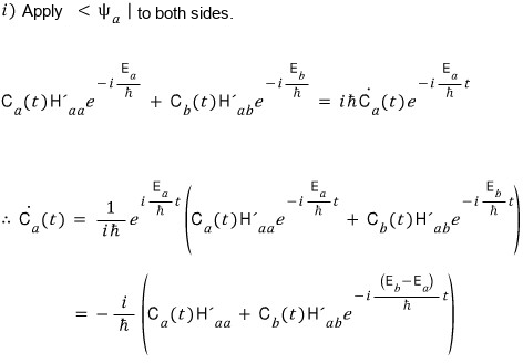
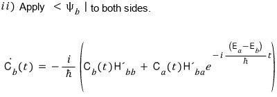
For the simplified model that follows, assume the diagonal elements vanish:

This is an assumption about the operator and the chosen basis, not a universal property of absorption or emission. It holds for an electric dipole perturbation between states of definite parity, because the position operator is odd under spatial inversion. If the diagonal elements are nonzero, the two preceding equations retain them.

Let $E_b>E_a$ and define the positive angular frequency $\omega_0=(E_b-E_a)/\hbar$. The equations reduce to

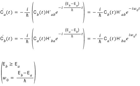
Hermiticity requires $H'_{ba}=(H'_{ab})^*$. It does not generally make the two matrix elements equal: equality additionally requires that the matrix element be real in the chosen phase convention. No expansion in the perturbation strength has been made in these two coupled equations.

Example 9.1: a hydrogen atom in an electric field

Consider a field directed along the $z$ axis:

Write its real, signed amplitude as $E(t)$. In the electric dipole approximation, the field is spatially uniform across the atom. With electron charge $-e$, where $e>0$, the interaction energy is $-\mathbf d\cdot\mathbf E=eE(t)z$:

We want the four matrix elements coupling the $1s$ ground state to the $n=2$ states:

We will also verify that each of the five states has a zero diagonal dipole matrix element:

Here we use the nonrelativistic Coulomb model, ignoring electron spin, fine structure, and the Lamb shift. In that model the first excited level has four spatial states. The five wavefunctions involved are

Their radial and angular factors are

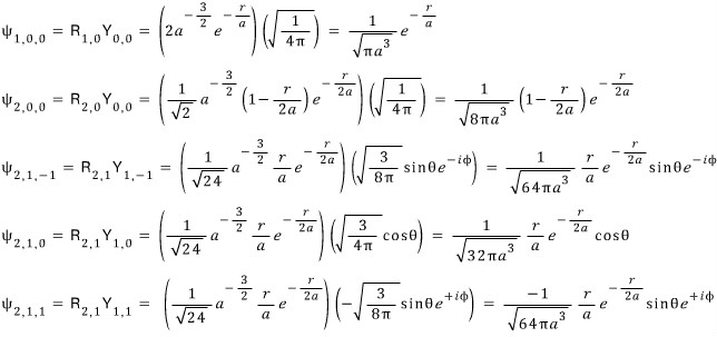
The symbol $a$ denotes the Bohr radius. We use the conventional phases $Y_1^{\pm1}\propto\mp\sin\theta\,e^{\pm i\phi}$ and a positive radial factor for the $2p$ states. These conventions agree with the hydrogen radial functions and spherical harmonics tabulated by Oregon State University. A consistent overall phase change of a basis state changes some matrix-element signs but leaves transition probabilities unchanged.

The interaction is a scalar energy operator, so its matrix elements contain $eE(t)z$:

Use reflection symmetry before integrating

For these integrals, reflect $z\to-z$ while holding $x$ and $y$ fixed. Since $r=\sqrt{x^2+y^2+z^2}$ does not change, every radial factor is even in $z$.

For example, the ground-state wavefunction is

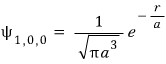
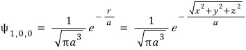
and its Cartesian form makes the symmetry explicit:

The radial factors of the $2p$ states contain a factor proportional to $r$ times a decaying exponential. Schematically, suppressing the fixed length scales,

Both factors remain unchanged under $z\to-z$. The $2s$ factor $(1-r/2a)$ is also even in $z$.

What distinguishes the three $2p$ states is their angular dependence:

The $m=\pm1$ states contain

whereas the $m=0$ state contains

Convert these combinations to Cartesian coordinates:

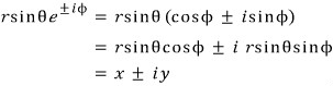
Thus the two states

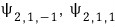
are even in $z$, because

has no explicit $z$ dependence. The remaining radial factor depends only on $r$ and is also even. By contrast,

is odd in $z$, because its angular and radial factors contain $r\cos\theta=z$.

The reflection properties are therefore

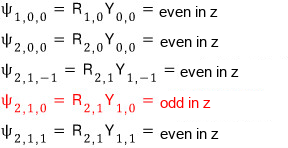
This is reflection in the $xy$ plane. It should not be confused with full spatial inversion, under which all three coordinates change sign and every $p$ orbital has odd parity.

Return to the matrix elements:

For a diagonal element, $\psi_i^*z\psi_i=z|\psi_i|^2$ is odd in $z$. Integration over all space gives zero:

For transitions from the ground state, the four spatial integrals are

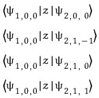
Because the $1s$ state is even in $z$, the $2s$ and $2p_{\pm1}$ integrands are odd and vanish. Only the $2p_0$ integral can survive:

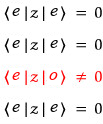
Here the letters $e$ and $o$ stand for even and odd functions, rather than electric charge. Evenness of an integrand permits a nonzero result; it does not by itself prove that the integral is nonzero. We still need to evaluate the surviving integral.

Evaluate the surviving dipole matrix element

Let $a$ label $1s$ and $b$ label $2p_0$. With the phases specified above, evaluate $H'_{ab}(t)=eE(t)\langle1s|z|2p_0\rangle$. At a fixed time, $E(t)$ is constant with respect to the spatial integration; it is abbreviated as $E$ in the working below:

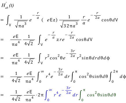
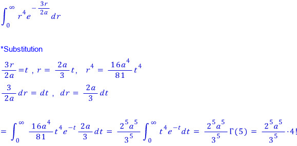
The radial integral becomes a gamma-function integral after setting $u=3r/(2a)$. The working uses $t$ as the dummy integration variable here; it is unrelated to physical time:

For the polar-angle integral, either set $u=\cos\theta$ or use the identity shown below:

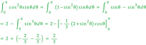
The antiderivative used in that calculation is

Combining the radial, polar, and azimuthal integrals gives

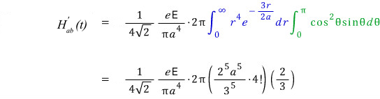
The compact result is

$$ \langle1s|z|2p_0\rangle=\frac{128\sqrt{2}}{243}\,a, \qquad H'_{ab}(t)=\frac{128\sqrt{2}}{243}\,e a E(t). $$

This has the expected units: the position matrix element is a length, and the perturbation matrix element is an energy. The other three ground-to-$n=2$ dipole matrix elements vanish. In this real basis and for a real field, $H'_{ba}=H'_{ab}$; more generally, the reverse element is its complex conjugate.

Starting from $1s$, only $2p_0$ acquires an amplitude at first order among these four excited states. That observation suggests a two-level approximation, but does not make it exact. The same operator also couples $2p_0$ to $2s$, and it couples to higher states. A weak field with a suitable frequency and bandwidth can make the omitted couplings negligible. Merely discarding states with $n>2$ is not sufficient to justify an exact two-state model.

Example 9.2: an exact solution for constant coupling

Now study the ideal two-level model itself. Take $H'_{aa}=H'_{bb}=0$, let the off-diagonal matrix elements be constant during the interval of interest, and impose the initial conditions

The atom starts entirely in state $a$. We will solve for both amplitudes and check normalization:

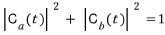
Although we introduced these equations in a discussion of perturbation theory, the solution below is exact within the two-level model. It does not assume that the transition probability stays small.

What changes when the Hamiltonian is constant?

With nonzero coupling, the system evolves from the pure lower basis state

into a superposition containing the upper basis state

This is compatible with a time-independent Hamiltonian. A state that is an eigenstate of that full Hamiltonian remains in the same energy eigenspace, up to a phase. But our basis states

and

are eigenstates of $H^0$, not of $H^0+H'$ when the off-diagonal coupling is nonzero. The energy labels

and

belong to $H^0$. Measuring the full Hamiltonian while the coupling is on gives its shifted eigenvalues,

$$ E_\pm=\frac{E_a+E_b}{2} \pm\frac{1}{2}\sqrt{(E_b-E_a)^2+4|H'_{ab}|^2}. $$

For a transition experiment, imagine switching the perturbation on and then off again. Before and after the pulse, the states

and

are again eigenstates of the actual Hamiltonian, $H^0$. Turn on a constant coupling at

and turn it off after a duration

The switching makes the complete pulse protocol time dependent, even though the Hamiltonian is constant during the pulse. The ideal sudden switch leaves the state continuous; a finite switching ramp would have its own dynamics. After switch-off, $|C_b(t)|^2$ is the probability of measuring the unperturbed upper energy.

Solve the coupled equations

The starting equations are

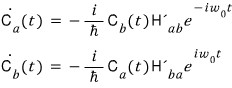
Our eventual goal is to find

but it is convenient to obtain $C_b(t)$ first. Differentiate the second equation and substitute the first. Since the matrix elements are constant, their time derivatives vanish. Hermiticity gives $H'_{ba}H'_{ab}=|H'_{ab}|^2$:

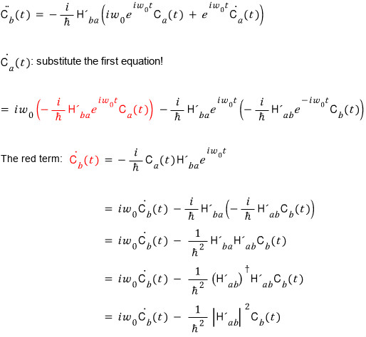
Define $\alpha=|H'_{ab}|/\hbar\geq0$. The resulting second-order equation is

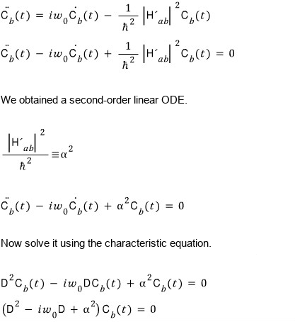
In the characteristic-equation method, $D$ represents the time derivative when acting on a function, and its characteristic roots are

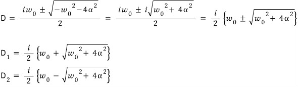
Let $\Omega=\sqrt{\omega_0^2+4\alpha^2}$. The two exponential solutions combine linearly; the initial condition $C_b(0)=0$ makes their coefficients equal and opposite:

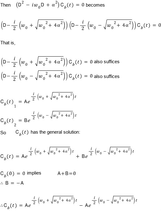
Use Euler’s formula to write the difference of exponentials as a sine:

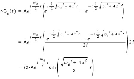
We now have the form of

with one undetermined constant $A$. Fix it using the original first-order equation

Differentiate the sine-form solution:

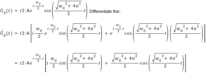
and equate the result to

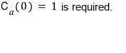
The remaining initial condition is

Solving the first-order equation for $C_a(t)$ gives

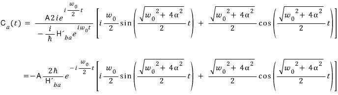
and evaluating at zero fixes $A$:

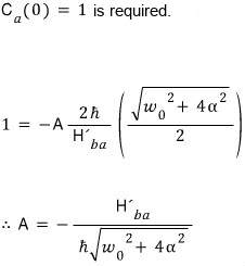
Substituting it back yields the lower-state amplitude

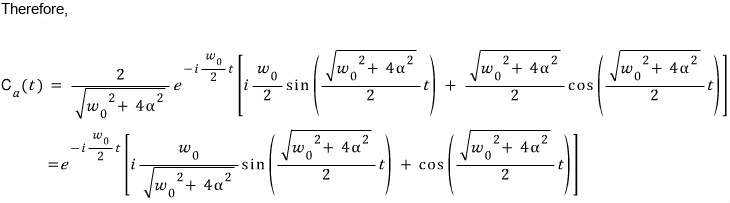
and the upper-state amplitude

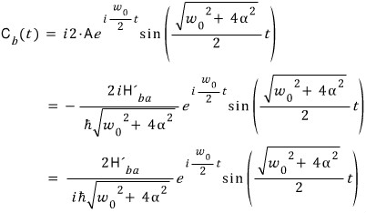
The algebra involving division by $H'_{ba}$ assumes nonzero coupling. When the coupling vanishes, the original equations immediately give $C_a(t)=1$ and $C_b(t)=0$.

Check the probabilities

To obtain probabilities, take the absolute square of each amplitude. The factors $e^{\pm i\omega_0t/2}$ have unit magnitude and disappear. The imaginary sine term and real cosine term in $C_a$ produce no cross term in its absolute square. The handwritten calculation abbreviates $\Omega t/2$ as $\phi$:

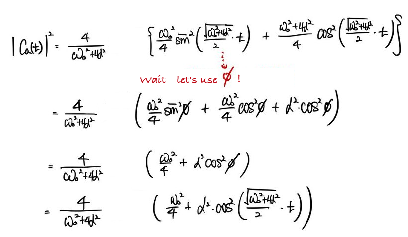
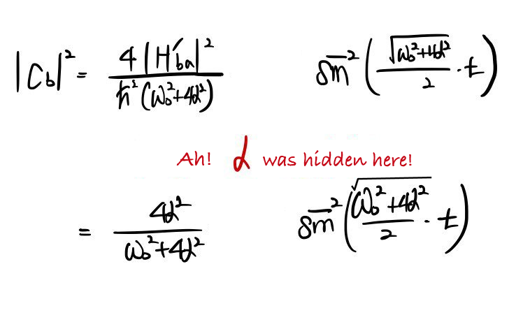
Adding the two probabilities confirms normalization at every time:

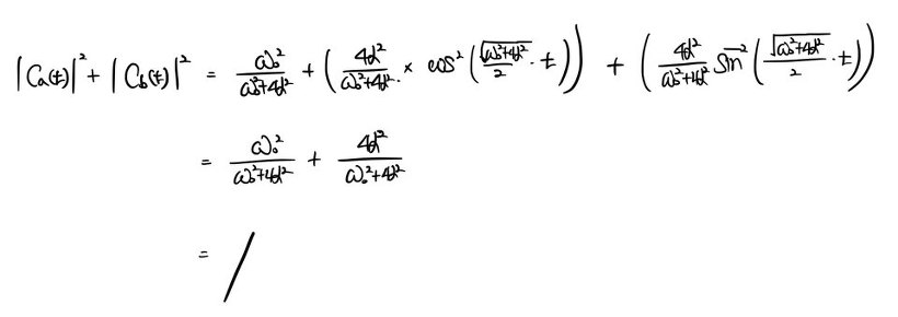
The upper-state population is $P_b(t)=(4\alpha^2/\Omega^2)\sin^2(\Omega t/2)$, with $P_a(t)=1-P_b(t)$. For separated unperturbed levels, its maximum is less than one. Complete transfer becomes possible in the degenerate limit $\omega_0=0$ of this constant-coupling model. The oscillations conserve the expectation value of the full Hamiltonian while the coupling is held constant; the populations of the unperturbed states need not be constant.

This distinction between a fixed Hamiltonian’s eigenstates and the basis used to describe the state is central to two-level dynamics. MIT’s notes on time-independent two-level Hamiltonians give a complementary matrix-based treatment. In the next post, an oscillating perturbation will connect these amplitude equations to absorption and stimulated emission.