Absorption, Emission, and Stimulated Emission

What happens when we shine light on an atom? The atom can absorb energy and move to a higher state, or an excited atom can transfer energy back to the light. Time-dependent perturbation theory lets us calculate both processes within the same framework.

Let’s start with a sinusoidal perturbation, then identify the interaction that describes an atom in an electric field. Throughout, we assume a weak perturbation and focus on two unperturbed states, $a$ and $b$, with $E_b>E_a$.

A sinusoidal perturbation

Take the perturbation Hamiltonian to be

Here $V(\mathbf r)$ is a time-independent operator. The applied angular frequency $\omega$ is adjustable; it is distinct from the fixed transition frequency $\omega_0=(E_b-E_a)/\hbar$. The equation images use $w$ for $\omega$.

We write the interaction between the two states in terms of matrix elements:

Suppose the atom begins in state $a$, so $C_a(0)=1$ and $C_b(0)=0$. These coefficients are probability amplitudes: the probabilities are $|C_a(t)|^2$ and $|C_b(t)|^2$.

More explicitly, our convention is

$$ |\Psi(t)\rangle=C_a(t)e^{-iE_at/\hbar}|a\rangle+C_b(t)e^{-iE_bt/\hbar}|b\rangle. $$

For now, take the diagonal perturbation matrix elements to vanish. We will justify that assumption for states of definite parity below. Substituting the unperturbed amplitudes into the coupled equations gives the first-order equations

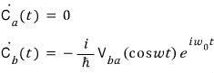
Integrating from $0$ to $t$ and expanding the cosine into two exponentials gives

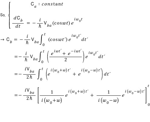
Inside the integral, use the Euler expansion $\cos(\omega t')=(e^{i\omega t'}+e^{-i\omega t'})/2$. After evaluating the integral, both exponents contain the upper limit $t$. The resulting amplitude is

$$ C_b^{(1)}(t)=-\frac{V_{ba}}{2\hbar} \left[ \frac{e^{i(\omega_0+\omega)t}-1}{\omega_0+\omega} +\frac{e^{i(\omega_0-\omega)t}-1}{\omega_0-\omega} \right]. $$

The superscript $(1)$ identifies the term that is first order in the perturbation. At this order, $C_a(t)\approx1$ and $C_b(t)\approx C_b^{(1)}(t)$.

Why a constant initial amplitude does not violate normalization

The exact amplitudes of a closed two-state system obey

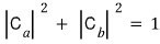
If we insert $C_a=1$ together with a nonzero $C_b^{(1)}$, the sum becomes $1+|C_b^{(1)}|^2$. The extra term is second order in the interaction strength. A calculation that keeps amplitudes only through first order has omitted the second-order change in $C_a$ that compensates for it.

Thus, when using the truncated amplitudes, the equality is approximate:

For the off-diagonal coupling assumed here, a consistent second-order calculation gives $2\operatorname{Re}C_a^{(2)}=-|C_b^{(1)}|^2$. The leading transition probability can therefore be found from the first-order amplitude, but the approximation requires that probability to remain small. Exact time evolution remains normalized. MIT’s treatment of perturbative amplitudes and transition probabilities gives the underlying expansion.

Resonance and the transition probability

The two terms in $C_b^{(1)}$ behave differently near resonance:

When $|\omega_0-\omega|\ll\omega_0+\omega$, the difference-frequency term varies slowly, while the sum-frequency term oscillates rapidly. For a weak drive observed over many optical cycles, retaining the slowly varying term captures the resonant response. A small denominator does not cause an actual divergence at fixed time: its numerator vanishes at the same point.

Retaining the difference-frequency term gives

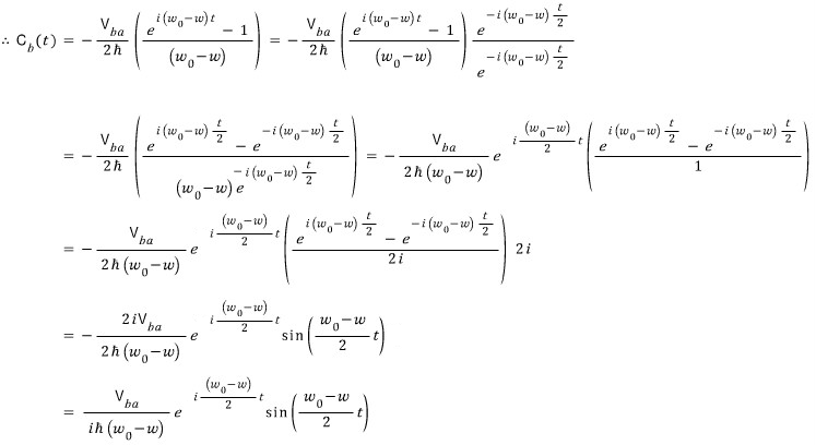
To express this amplitude as a sine, define $\Delta=\omega_0-\omega$. The identity $e^{i\Delta t}-1=2i e^{i\Delta t/2}\sin(\Delta t/2)$ gives

$$ C_b^{(1)}(t)\approx-\frac{iV_{ba}}{\hbar}\, e^{i\Delta t/2}\frac{\sin(\Delta t/2)}{\Delta}. $$

Because the atom started in state $a$, $|C_b^{(1)}(t)|^2$ is the leading probability for the transition $a\to b$. Multiplication by the complex conjugate removes the phase factor, giving

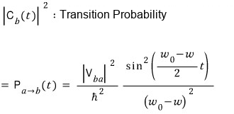
At fixed interaction time, this is a sharply peaked function of the applied frequency:

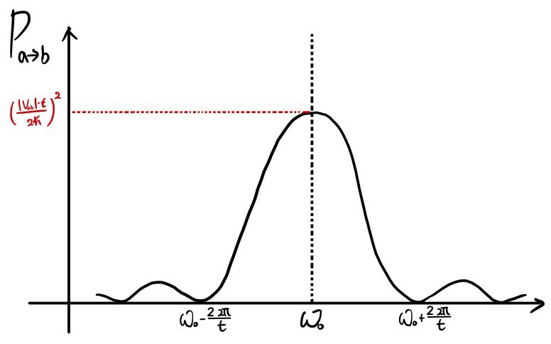
The first zeros occur where $\Delta t/2=\pm\pi$, so their correct frequencies are $\omega_0\pm2\pi/t$. The width between the first zeros is therefore $4\pi/t$, as stated in the next image.

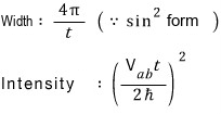
The quantity labeled “Intensity” here is the peak transition probability, not the optical intensity. In general it is $|V_{ba}|^2t^2/(4\hbar^2)$; the ordinary square shown in the image assumes a real matrix element. This peak follows from the finite limit $\sin(\Delta t/2)/\Delta\to t/2$ as $\Delta\to0$.

Longer interaction times produce a narrower frequency response. The following annotations summarize the ideal resonance condition:

At finite time, the transition probability can be nonzero away from resonance. The sharp energy-selection condition belongs to an ideal long-time limit used in deriving transition rates. Even then, we cannot extrapolate the resonant $t^2$ probability indefinitely: eventually the small-transition-probability approximation fails.

Fermi’s golden rule combines this energy selection with a continuum, or sufficiently dense set, of final states to obtain a transition rate. A coherently driven isolated two-level system requires its own time evolution once the first-order approximation breaks down. Fitzpatrick’s discussion of harmonic perturbations distinguishes transition amplitudes from continuum transition rates. We will develop the golden-rule calculation in the next post.

What the two-level picture represents

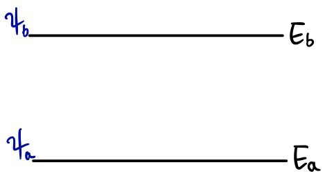
An atom generally has many energy levels; the two-level model retains a selected pair. A dilute atomic gas is a useful setting in which to picture separate atomic transitions. This does not mean that every system with discrete levels must be a gas. In a solid, interactions between atoms can produce energy bands, so its optical response often requires more states than this simple diagram includes. MIT’s introduction to band theory explains how bands arise from atomic levels.

Light as an electric dipole perturbation

We can now make $V(\mathbf r)$ concrete by considering an atom illuminated by light. Here the atom is quantum mechanical and the applied electromagnetic field is classical.

Light has both electric and magnetic fields. We retain the electric dipole interaction, which is the leading contribution for the allowed transitions considered here. Magnetic interactions are separate, weaker contributions in this setting; the existence of a related electric field is not, by itself, a reason to discard them.

We write the oscillating electric field as

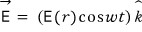
The unit vector $\hat{\mathbf k}$ in these images denotes the polarization direction, chosen below to be $\hat{\mathbf z}$. It is not the light’s propagation direction. For a plane wave in free space, the electric field is transverse to propagation.

The electric dipole approximation

If the wavelength is much larger than the atomic size $a$, the field changes very little across the atom:

More precisely, we require $2\pi a/\lambda\ll1$. We then evaluate the field at the atom’s position and neglect its variation across the electronic wavefunction:

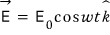
This is the electric dipole approximation. The atom still interacts with the field; the approximation removes the field’s spatial variation across the atom. We also assume monochromatic light, a fixed linear polarization along $z$, and a prescribed applied field whose depletion we neglect. MIT’s light–matter interaction notes derive the long-wavelength approximation.

The interaction energy and transition dipole

For a signed charge $q$, define the electric dipole operator as $\mathbf d=q\mathbf r$. In the electric dipole approximation,

$$ H'(t)=-\mathbf d\cdot\mathbf E(t)=-qzE_0\cos(\omega t), \qquad V(\mathbf r)=-qE_0z. $$

We can also obtain this interaction energy by integrating the force along the $z$ direction:

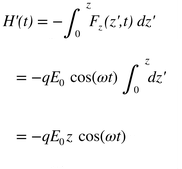
Since $F_z=qE_0\cos(\omega t)$, the corresponding energy change is $-\int_0^zF_z\,dz'=-qE_0z\cos(\omega t)$. For an electron, $q=-e$, where $e>0$, this becomes $+eE_0z\cos(\omega t)$. Either notation works if the charge convention is used consistently. The electric dipole interaction is $-\mathbf d\cdot\mathbf E$. MIT light–matter notes, equation 4.44.

Taking the matrix element gives

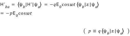
The symbol $p$ here denotes the transition dipole matrix element $p=q\langle b|z|a\rangle$. The coefficient of $\cos(\omega t)$ is therefore

In other words, $V_{ba}=-pE_0$, which has the required units of energy. The matrix element $\langle b|z|a\rangle$ determines how strongly the two states couple to the field.

Substituting this coefficient into the transition probability gives

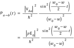
The overall sign disappears upon taking the modulus squared. The transition strength depends on $|p|^2E_0^2$, while the detuning controls the frequency response.

Parity and Hermiticity are different conditions

For an inversion-symmetric unperturbed Hamiltonian, we can choose states of definite parity. Their spatial wavefunctions,

are then even or odd under $\mathbf r\to-\mathbf r$. Because $z$ is odd, each diagonal expectation value $\langle i|z|i\rangle$ vanishes. Consequently,

This supplies the assumption used at the start. The same parity argument shows that an electric dipole matrix element between two states of the same parity is zero. Opposite parity is necessary, but other selection rules can still make a transition vanish. Fitzpatrick’s electric dipole discussion develops these restrictions further.

For real matrix elements, we also have

This relation follows from Hermiticity together with the choice of real matrix elements. More generally, Hermiticity gives $V_{ab}=V_{ba}^{*}$, regardless of parity. Consequently, $|V_{ab}|^2=|V_{ba}|^2$, which is all we need when comparing the transition probabilities.

Stimulated emission

Now prepare the atom in the upper state instead:

Repeating the first-order calculation gives the downward transition probability

which equals the upward transition probability for the same pair of states, drive, and interaction time:

The equality follows because reversing the transition complex-conjugates the relevant first-order amplitude, up to an irrelevant sign. The upward process is absorption: energy passes from the field to the atom. The downward process caused by the applied field is stimulated emission: energy passes from the excited atom to the field. The equality here concerns a specified pair of states at this perturbative order, not the total absorption and emission of a sample with arbitrary level populations. MIT’s first-order reciprocity relation states this equality directly.

Stimulated emission supplies the amplification mechanism in a laser. LASER stands for Light Amplification by Stimulated Emission of Radiation. Producing net gain also requires a suitable population of excited atoms; equal probabilities for individual upward and downward transitions do not by themselves produce amplification. MIT’s radiation-interaction notes discuss this population requirement.

Spontaneous emission

An excited atom can also emit a photon without an applied driving field:

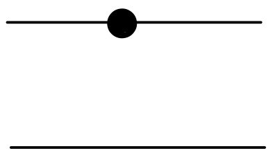
This process is spontaneous emission. The photon carries away the energy lost by the atom. Setting the classical driving field to zero in our calculation gives no transition, so this model does not explain spontaneous emission.

A quantum treatment includes the electromagnetic field as part of the system. An excited atom coupled to a field initially in its vacuum state can make a transition to a lower atomic state while creating a photon. Thus, spontaneous emission does not require thermal photons or an external light beam. The released energy comes from the atom’s excitation. MIT’s quantized-field treatment separates spontaneous and stimulated contributions.

The vacuum is the field’s lowest-energy quantum state. Its quantum fluctuations persist even in the absence of thermal radiation. This does not supply free energy to the emitted photon: the atom loses the corresponding excitation energy. The distinction between zero-point and thermal field energy is discussed in MIT’s notes on field quantization.

In the next post, we will examine Fermi’s golden rule and selection rules more closely. A later post will return to spontaneous emission through Einstein’s coefficients.