Chapter 9 Worked Problems: Time-Dependent Perturbations

These three Chapter 9 problems put time-dependent perturbation theory to work. First, we solve a sudden kick in a two-state system exactly. Next, we derive the corresponding amplitude equations for many states. Finally, we use the first-order result to find how a temporary potential excites a particle in an infinite square well.

The common thread is to follow probability amplitudes carefully. Their phases matter when we solve the equations, while their squared magnitudes give measurement probabilities. We also need to distinguish an exact result from an approximation that retains only the first few powers of the perturbation.

Problem 9.3: A delta-function pulse

The system begins in state $a$. A perturbation acts at $t=0$, coupling it to state $b$. Find the amplitudes after the pulse, check normalization, and calculate the transition probability.

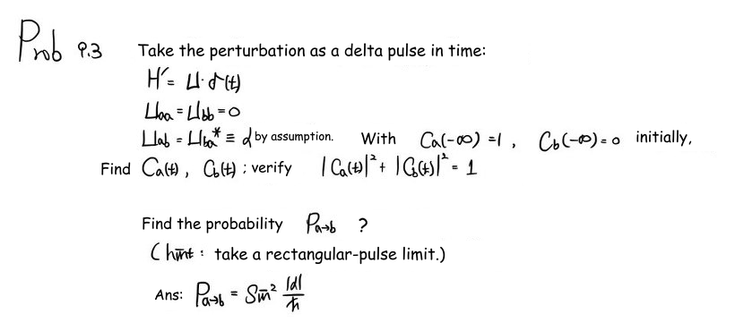
Let $H'(t)=U\delta(t)$, with diagonal matrix elements of $U$ equal to zero. The question defines

$$ U_{ab}=\alpha,\qquad U_{ba}=\alpha^*. $$

The star matters: $\alpha$ can be complex, and Hermiticity requires the two off-diagonal elements to be conjugates. Because $\delta(t)$ has units of inverse time, $U$ and $\alpha$ have units of action.

Replace the impulse by a narrow rectangle

It helps to picture a pulse whose area remains one as its width shrinks.

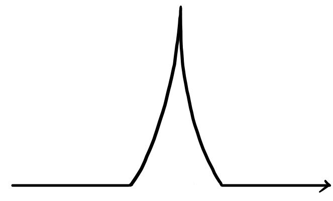
Unit area alone does not make an ordinary function a Dirac delta. We need a limiting family that becomes concentrated at $t=0$. Here the convenient choice is

$$ \delta_\epsilon(t)= \begin{cases} 1/(2\epsilon),& |t|<\epsilon,\\ 0,& |t|>\epsilon. \end{cases} $$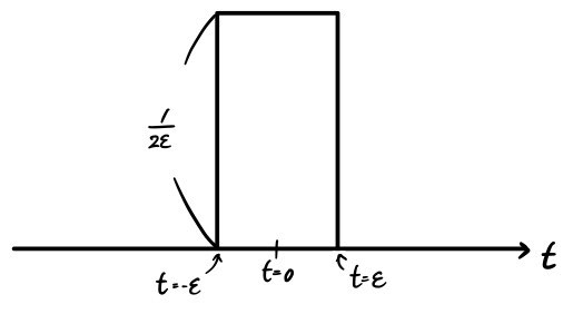

We solve the finite pulse first and then take $\epsilon\to0$. The height $1/(2\epsilon)$ belongs to the rectangle; it is not a finite value assigned to $\delta(0)$. This procedure also avoids trying to insert a single value of an amplitude into a delta integral when that amplitude changes across the pulse.

Before the pulse, $C_a=1$ and $C_b=0$. After it, both interaction-picture amplitudes are constant, but they need not be equal.

Our phase convention is

$$ |\Psi(t)\rangle= \sum_{n=a,b}C_n(t)e^{-iE_nt/\hbar}|n\rangle, $$

and $\omega_0=(E_b-E_a)/\hbar$. During the pulse the coupled equations are

$$ \dot C_a=-\frac{i\alpha}{2\hbar\epsilon} e^{-i\omega_0t}C_b, $$$$ \dot C_b=-\frac{i\alpha^*}{2\hbar\epsilon} e^{i\omega_0t}C_a. $$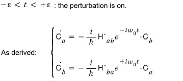

The opposite frequency phases follow from the opposite energy differences. The matrix element separates into a time factor and a state-space matrix element:

$$ H'_{ab}(t)=\delta_\epsilon(t)\langle a|U|b\rangle. $$

Thus, inside the rectangle, $H'_{ab}=\alpha/(2\epsilon)$ and $H'_{ba}=\alpha^*/(2\epsilon)$. If we write a spatial integral, it belongs to $\langle a|U|b\rangle$ and includes the conjugated bra wavefunction and the spatial integration measure.

The setup is the same one developed in time-dependent perturbation theory, Part 38. The absorption and stimulated-emission example in Part 39 uses a sinusoidal drive; here we keep the rectangular pulse and solve its coupled equations exactly.

Solve the finite pulse

Differentiate the equation for $C_b$ once more, then substitute the equation for $\dot C_a$.

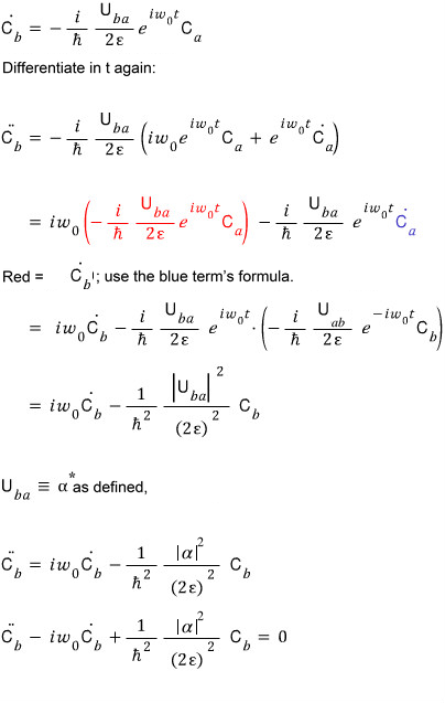
The result is

$$ \ddot C_b-i\omega_0\dot C_b +\frac{|\alpha|^2}{4\hbar^2\epsilon^2}C_b=0. $$

The product of the two couplings is $\alpha^*\alpha=|\alpha|^2$. Define the real, nonnegative frequency

$$ \Omega_\epsilon= \sqrt{\omega_0^2+\frac{|\alpha|^2}{\hbar^2\epsilon^2}}. $$

I will shorten this to $\Omega$ within the finite-pulse calculation. It is the quantity denoted by $w$ in the working below; $w_0$ denotes $\omega_0$.

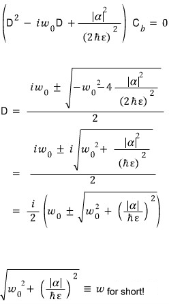
The roots are $i(\omega_0+\Omega)/2$ and $i(\omega_0-\Omega)/2$, so

$$ \begin{aligned} C_b(t)={}&A e^{i(\omega_0+\Omega)t/2}\\ &+B e^{i(\omega_0-\Omega)t/2}. \end{aligned} $$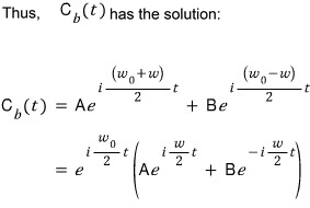

The first boundary condition, $C_b(-\epsilon)=0$, gives $B=-A e^{-i\Omega\epsilon}$.

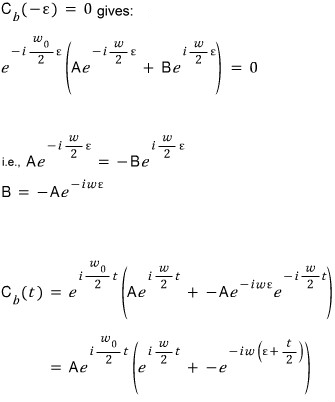
To determine $A$, differentiate this general solution and compare it with the original first-order equation for $\dot C_b$.

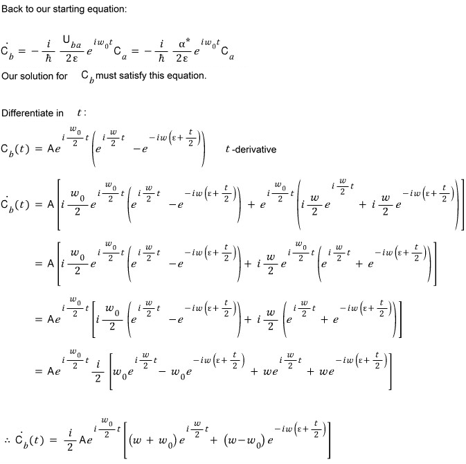
That equation also gives $C_a$ in terms of the derivative of $C_b$:

$$ C_a(t)=\frac{2i\hbar\epsilon}{\alpha^*} e^{-i\omega_0t}\dot C_b(t). $$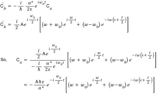

For nonzero $\alpha$, imposing $C_a(-\epsilon)=1$ gives

$$ A=-\frac{\alpha^*}{2\hbar\epsilon\Omega} e^{i(\Omega-\omega_0)\epsilon/2}. $$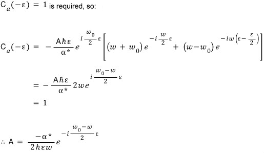

The exponentials become easier to read as sines and cosines. Define the short phase variables

$$ s=\frac{\Omega(t+\epsilon)}{2},\qquad \chi_\pm=\frac{\omega_0(t\pm\epsilon)}{2}. $$

Then the lower-state amplitude is

$$ C_a(t)=e^{-i\chi_+} \left(\cos s+i\frac{\omega_0}{\Omega}\sin s\right). $$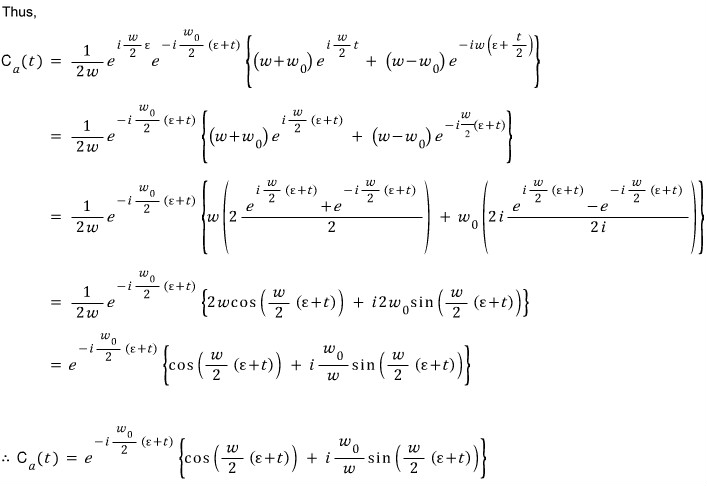

Similarly,

$$ C_b(t)=-\frac{i\alpha^*}{\hbar\epsilon\Omega} e^{i\chi_-}\sin s. $$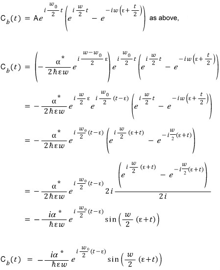

At the end of the rectangle, $t=\epsilon$, these expressions become

$$ C_a(\epsilon)=e^{-i\omega_0\epsilon} \left[\cos(\Omega\epsilon) +i\frac{\omega_0}{\Omega}\sin(\Omega\epsilon)\right], $$$$ C_b(\epsilon)=-\frac{i\alpha^*}{\hbar\epsilon\Omega} \sin(\Omega\epsilon). $$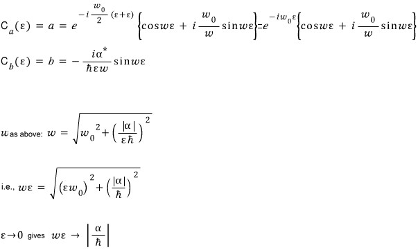

Take the delta limit and check the probability

As $\epsilon\to0$, we have $\epsilon\Omega\to|\alpha|/\hbar$. For $\alpha\ne0$, the amplitudes after the impulse are therefore

$$ C_a=\cos\left(\frac{|\alpha|}{\hbar}\right), $$$$ C_b=-i\frac{\alpha^*}{|\alpha|} \sin\left(\frac{|\alpha|}{\hbar}\right). $$

At $\alpha=0$, use the continuous result $C_a=1$, $C_b=0$; there is no coupling and no transition.

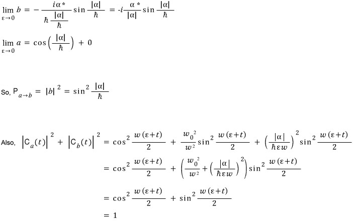
We can check normalization even before taking the limit. Set

$$ q=\frac{\omega_0}{\Omega},\qquad g=\frac{|\alpha|}{\hbar\epsilon\Omega}. $$

The definition of $\Omega$ gives $q^2+g^2=1$, and hence

$$ |C_a|^2+|C_b|^2 =\cos^2s+(q^2+g^2)\sin^2s=1. $$

The desired transition probability is

$$ P_{a\to b}=\sin^2\left(\frac{|\alpha|}{\hbar}\right). $$

There is also a compact operator check. Since $U^2=|\alpha|^2I$, the impulse applies the unitary operator $K=e^{-iU/\hbar}$. Acting on the initial state gives the same cosine and sine amplitudes. This is an exact impulse result, with no assumption that $|\alpha|/\hbar$ is small. Only in the weak-kick limit does it reduce to $P_{a\to b}\approx|\alpha|^2/\hbar^2$. MIT’s treatment of the delta-function perturbation provides a useful comparison.

Problem 9.15: Transition amplitudes for many states

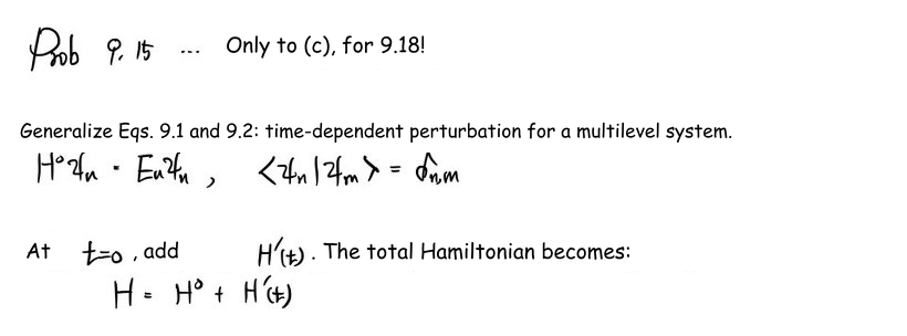
Now let the unperturbed Hamiltonian have an orthonormal energy basis $|n\rangle$. The goal is to generalize the two-state equations and then use them for a weak perturbation. Parts (a) through (c) supply the result needed for Problem 9.18.

Project the Schrödinger equation onto one state

Expand the state as

$$ |\Psi(t)\rangle= \sum_n C_n(t)e^{-iE_nt/\hbar}|n\rangle. $$

Substitute this expansion into the time-dependent Schrödinger equation. The terms containing $H_0|n\rangle=E_n|n\rangle$ cancel the derivatives of the free-evolution phases.

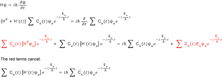
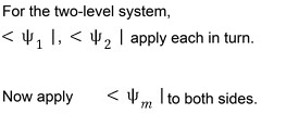
In a two-state calculation, we project onto $\langle a|$ and $\langle b|$. For many states, simply project onto an arbitrary $\langle m|$.

Orthogonality gives $\langle m|n\rangle=\delta_{mn}$, leaving one coefficient on the time-derivative side.

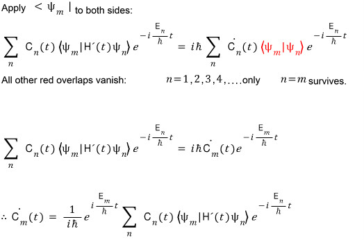
For clear order bookkeeping, write $H=H_0+\lambda V(t)$. Here $\lambda$ is a formal expansion parameter; the physical perturbation is recovered at $\lambda=1$. Define

$$ V_{mn}(t)=\langle m|V(t)|n\rangle, $$$$ W_{mn}(t)=V_{mn}(t)e^{i(E_m-E_n)t/\hbar}. $$

The exact coupled equations are then

$$ i\hbar\dot C_m(t)=\lambda\sum_n W_{mn}(t)C_n(t). $$

The $W_{mn}$ are the interaction-picture matrix elements. They package the energy-difference phases without changing the physics.

Keep the perturbative orders separate

Suppose the system starts in state $N$ at $t=0$. Only that initial amplitude is one; every other initial amplitude is zero.

Expand each amplitude as

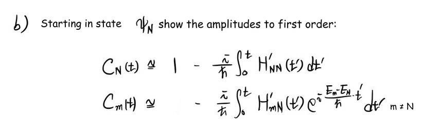
$$ C_m=C_m^{(0)}+\lambda C_m^{(1)} +\lambda^2 C_m^{(2)}+\cdots. $$

The initial conditions imply $C_m^{(0)}=\delta_{mN}$ and $C_m^{(k)}(0)=0$ for every $k\ge1$. At zeroth order, the interaction-picture coefficients stay at their initial values.

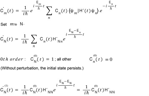
Substituting those zeroth-order coefficients into the right-hand side gives

$$ C_m^{(1)}(t)=-\frac{i}{\hbar} \int_0^t W_{mN}(t_1)\,dt_1. $$

In particular, $C_N^{(1)}$ has zero integration constant. The total amplitude through first order is $C_N\approx1+\lambda C_N^{(1)}$. The correction itself does not include that initial one.

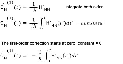
For $m\ne N$, the zeroth-order amplitude vanishes, so $C_m\approx\lambda C_m^{(1)}$. Written without the shorthand $W$, its integrand is $V_{mN}(t_1)e^{i(E_m-E_N)t_1/\hbar}$. Both time-dependent factors use the integration variable.

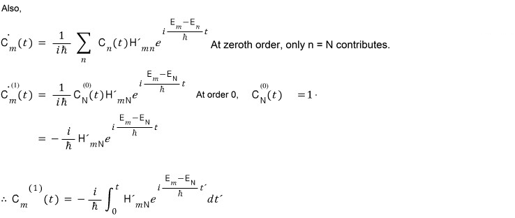
After integration, the result is an amplitude $C_m^{(1)}$, not its time derivative. A probability is dimensionless and comes from an amplitude’s squared magnitude.

A second-order check on normalization

The same substitution can be repeated. The next correction includes an intermediate state $n$ and two ordered interaction times:

$$ \begin{aligned} C_m^{(2)}(t)={}&-\frac{1}{\hbar^2}\sum_n \int_0^t dt_1\int_0^{t_1}dt_2\\ &\times W_{mn}(t_1)W_{nN}(t_2). \end{aligned} $$

The earlier interaction occurs at $t_2$ and the later one at $t_1$. Because the region already enforces $0\le t_2\le t_1\le t$, no extra factor of $1/2$ is needed. This is the second-order term of the Dyson expansion.

For a Hermitian perturbation, $\operatorname{Re}C_N^{(1)}=0$, and normalization through second order requires

$$ 2\operatorname{Re}C_N^{(2)} +\sum_m|C_m^{(1)}|^2=0. $$

The second-order change in the survival amplitude compensates for the leading transition probabilities. Keeping $C_N=1$ while adding nonzero first-order amplitudes to other states only satisfies normalization to first order. Exact evolution is still unitary.

A perturbation that stays constant for a finite time

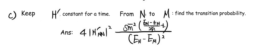
Set $\lambda=1$ again. Suppose $V$ is constant during the interval being considered, and consider a transition from $N$ to $M\ne N$.

Write $\Delta E=E_M-E_N$. For a nonzero gap, the first-order integral gives

$$ C_M^{(1)}(t)= \frac{V_{MN}}{\Delta E} \left(1-e^{i\Delta E t/\hbar}\right). $$

Equivalently,

$$ C_M^{(1)}(t)=-\frac{2iV_{MN}}{\Delta E} e^{i\Delta E t/(2\hbar)} \sin\left(\frac{\Delta E t}{2\hbar}\right). $$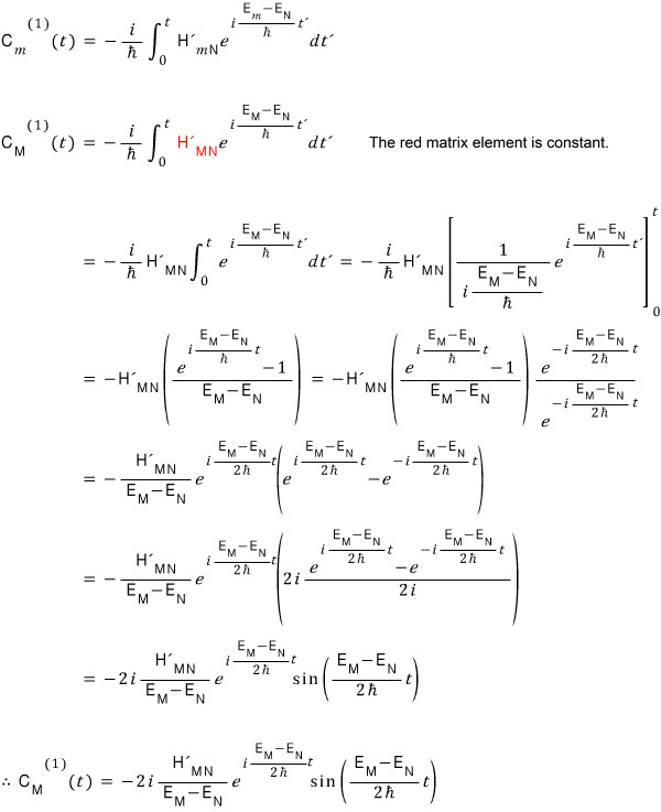

Taking the squared magnitude removes the pure phase:

$$ P_{N\to M}(t)\approx \frac{4|V_{MN}|^2}{(\Delta E)^2} \sin^2\left(\frac{\Delta E t}{2\hbar}\right). $$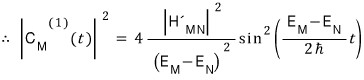

Although the amplitude is first order in $V$, this leading transition probability is second order in its strength. The apparent zero-gap singularity is removable: as $\Delta E\to0$, the amplitude approaches $-iV_{MN}t/\hbar$, and the leading probability approaches $|V_{MN}|^2t^2/\hbar^2$.

These approximations require neglected amplitude corrections to remain small. In particular, the transition probabilities must be small; extending the formula to arbitrarily long times near degeneracy is not justified. We have calculated a finite-time probability between discrete states, not an irreversible transition rate. The constant-perturbation calculation is also discussed in the University of Texas quantum-mechanics notes.

Problem 9.18: Temporarily raise half of an infinite well

Now use the previous result in a spatial problem. A particle of mass $m$ starts in the ground state of an infinite well extending from $x=0$ to $x=a$. At $t=0$, raise the potential in the left half by $V_0$. Remove this perturbation after a time $T$, then measure the energy. What is the probability of obtaining $E_2$?

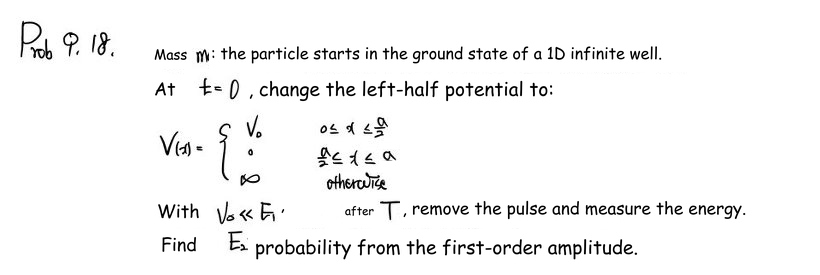
Inside the well and during $0\lt t\lt T$, the added potential is $V_0$ for $0\lt x\lt a/2$ and zero for $a/2\lt x\lt a$. The infinite walls remain in place. We assume $|V_0|\ll E_1$ and use a first-order amplitude calculation.

The unperturbed states and energies are

$$ \psi_n(x)=\sqrt{\frac{2}{a}}\sin\left(\frac{n\pi x}{a}\right), $$$$ E_n=\frac{n^2\pi^2\hbar^2}{2ma^2}. $$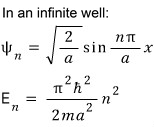

These are the eigenstates of the original well, so they are also the energy-measurement states after the perturbation has been removed. See MIT’s infinite-square-well notes for the normalization and spectrum.

The initial condition is $C_n(0)=\delta_{n1}$. It is the ground-state zeroth-order amplitude that equals one, not every first-order correction.

The pulse is constant in time until it is removed, so we can use the result from Problem 9.15 and evaluate it at $t=T$.

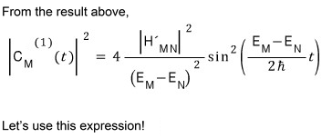
With $N=1$ and $M=2$, define $\Delta E_{21}=E_2-E_1$. Then

$$ P_{1\to2}(T)\approx \frac{4|V_{21}|^2}{(\Delta E_{21})^2} \sin^2\left(\frac{\Delta E_{21}T}{2\hbar}\right). $$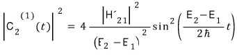

The energy gap is straightforward:

$$ \Delta E_{21}=\frac{3\pi^2\hbar^2}{2ma^2}. $$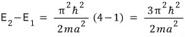

The remaining task is the matrix element. Only the left half contributes:

$$ V_{21}=\frac{2V_0}{a}\int_0^{a/2} \sin\left(\frac{2\pi x}{a}\right) \sin\left(\frac{\pi x}{a}\right)\,dx. $$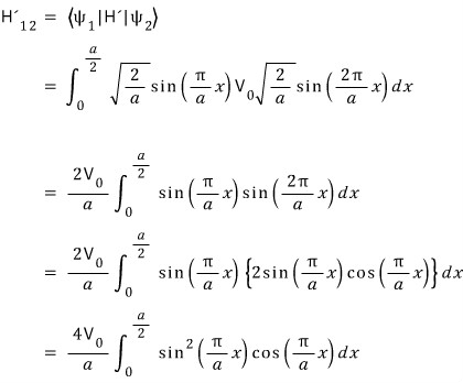

Use $\sin(2\theta)=2\sin\theta\cos\theta$, then substitute $u=\sin(\pi x/a)$. The integration limits become zero and one. I use $u$ here to keep this dummy variable distinct from physical time.

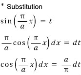
The integral reduces to

$$ V_{21}=\frac{4V_0}{\pi}\int_0^1u^2\,du =\frac{4V_0}{3\pi}. $$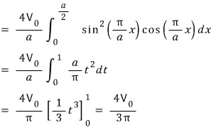

Substituting the gap and matrix element gives

$$ P_{1\to2}(T)\approx \left[ \frac{16ma^2V_0}{9\pi^3\hbar^2} \sin\left(\frac{3\pi^2\hbar T}{4ma^2}\right) \right]^2. $$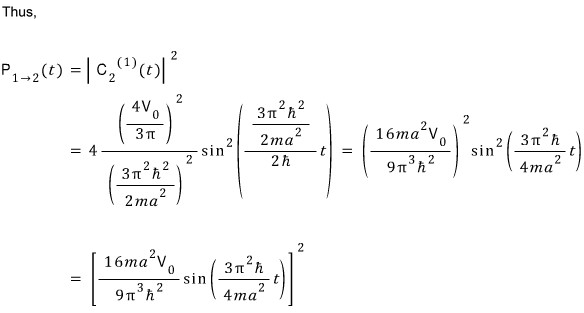

The square applies to the entire bracket. It makes the probability nonnegative and quadratic in the weak potential. At $V_0=0$ or $T=0$, the probability vanishes, as it should. The sine describes interference between transition amplitudes accumulated during the finite pulse.

After $t=T$, the interaction-picture coefficients stop changing, so the energy probabilities remain at their switch-off values. The components of the physical state still acquire their usual free-evolution phases. This result is the leading weak-potential probability, valid while omitted perturbative corrections remain negligible; it is not an exact solution for an arbitrarily strong or long pulse.

A note on the equations. My original working contained inconsistent phase signs, conjugates, derivative dots, and perturbative-order notation. The derivation in this English edition keeps $U_{ba}=\alpha^*$, separates a first-order correction from the initial amplitude, and uses squared amplitudes for probabilities. In the normalization check, the frequency ratio is squared as well. The final square-well probability already has the required outer square; the time in that formula is evaluated at the pulse duration $T$.