Derivation of the Exponential Distribution [Basic Statistics I Studied #3]

Since we covered the Poisson distribution earlier, the 'normal distribution', or Gaussian distribution, should actually come next in order.

But I will skip the normal distribution!!!!

We are doing the exponential distribution!!

As you probably noticed while solving problems involving the Poisson distribution,

or, well, rather than noticing, should I say you felt it in your heart?

Anyway, the Poisson distribution

was a distribution of "the number of events occurring during a specified time interval."

Then this exponential distribution here concerns "the waiting time until the first event occurs during a specified time interval."

Then, in a Poisson distribution with an average of λ occurrences per unit interval,

$f(x)=\frac{\lambda^x e^{-\lambda}}{x!}$ I will extend the interval!!!

Then we extend it to "interval t", and how many occurrences would we expect on average in this interval?

The average per unit time was λ events,

so "per interval t" the average would be λt. <This is included in the assumptions of the Poisson distribution.>

Then the probability distribution function

$\frac{\lambda^x e^{-\lambda}}{x!}\ \rightarrow\ \frac{\lambda t^x e^{-\lambda t}}{x!}$ changes like this (still a Poisson distribution)

But let us put in x=0

\[p(x=0)=\frac{\lambda t^0 e^{-\lambda t}}{0!}=e^{-\lambda t}\]

$e^{-\lambda t}$ What this means is the probability of no event occurring during "interval t"....

That is, it means the same as "the probability that the waiting time until the first occurrence is t"!!!!

Conversely, the probability of an event occurring 'at least once' during interval t would be $1-e^{-\lambda t}$ like this....

Here, let us call the random variable representing "the waiting time (until the first occurrence)" time T, and think about that thing above once more

"The probability of no event occurring during interval t"

→ "The probability that T (the waiting time until the first occurrence) is greater than t"

→ As a formula: $p(T>t)$

→ Above, we said $e^{-\lambda t}$ , and therefore $p(T>t)=e^{-\lambda t}$:

Then,

"The probability of an event occurring at least once during interval t"

→ "The probability that T (the waiting time until the first occurrence) is less than t"

→ As a formula: $p(T\le t)$

→ Above, we said $1-e^{-\lambda t}$ , and therefore $p(T\le t)=1-e^{-\lambda t}$

$p(T\le t)$ is the cumulative probability distribution, right??!??!!?

I will write it like this

$\text{Cumulative probability distribution}=1-e^{-\lambda t}$

(differentiate it)

$\text{Probability density function}=\lambda e^{-\lambda t}$

is what we get. And this is what we call the exponential distribution >_<

What did it mean????????????????

The probability that the waiting time is t is what it would be

Oh (t and λ are positive!)

I will calculate the mean and variance of the exponential distribution.

Typing all of it into an equation editor would take a while,.... so, with a photo

But with a "pretty" photo... I will do it! Haha

And since we learned the moment generating function

it is simple because we will use that!!!!

(Of course, doing this one by integration is quite manageable too!!!! http://gdpresent.blog.me/220582073367 here it is!!!!)

Here below, with the moment generating function

we will pull out the mean and variance!!!!!!!!

I will temporarily call the random variable t (time) just x.

This is so we can keep using t as t, just as we did for the moment generating function

so please note that t below this point is not time

and below, f(x) is the exponential distribution whose random variable is time~~~

$f(x)=\lambda e^{-\lambda x}\quad(x>0,\ \lambda>0).$

Continuing with the moment generation function.

$M(t)=\int_0^\infty e^{tx}\cdot f(x)\cdot dx=\int_0^\infty e^{tx}\lambda e^{-\lambda x}dx=\int_0^\infty\lambda e^{(t-\lambda)x}\cdot dx.$

$=\int_0^\infty\lambda\cdot e^{-(\lambda-t)x}dx.=\left[-\frac{\lambda}{\lambda-t}e^{-(\lambda-t)x}\right]_0^\infty=\frac{\lambda}{\lambda-t}$

$M^{\prime}(t)=\frac d{dt}\cdot\frac{\lambda}{\lambda-t}=\frac{-(-\lambda)}{(\lambda-t)^2}=\frac\lambda{(\lambda-t)^2}$

$M^{\prime}(0)=\frac\lambda{\lambda^2}=\frac1\lambda=\mu=E(x).$

Mean

$M^{\prime\prime}(0)=\frac d{dt}\cdot M^{\prime}(t)=\frac d{dt}\frac\lambda{(\lambda-t)^2}=\frac{-\lambda\cdot\bigl(2\cdot(\lambda-t)\cdot(-1)\bigr)}{(\lambda-t)^4}=\frac{2\lambda}{(\lambda-t)^3}$

cf. It would be easier to differentiate it as a product:

$\frac d{dt}M^{\prime}(t)=\frac d{dt}\cdot\lambda\cdot(\lambda-t)^{-2}=-2\lambda(\lambda-t)^{-3}\cdot(-1)$

$=\frac{2\lambda}{(\lambda-t)^3}$

$M^{\prime\prime}(0)=\frac{2\lambda}{\lambda^3}=\frac2{\lambda^2}=E(x^2)$

$\therefore\ \sigma^2=E(x^2)-[E(x)]^2=\frac2{\lambda^2}-\left(\frac1\lambda\right)^2=\frac1{\lambda^2}$

Variance.

↓ Revised a little more prettily on the iPad

Let us pull out the mean and variance of the exponential distribution using the moment generating function.

$M(t)=\int_0^\infty e^{tx}f(x)\cdot dx$

$=\int_0^\infty e^{tx}\cdot\lambda e^{-\lambda x}dx$

$=\int_0^\infty\lambda e^{(t-\lambda)x}dx$

$=\int_0^\infty\lambda e^{-(\lambda-t)x}dx$

$=\left[-\frac{\lambda}{\lambda-t}e^{-(\lambda-t)x}\right]_0^\infty$

$=0-\left(-\frac{\lambda}{\lambda-t}\right)$

$=\frac{\lambda}{\lambda-t}$

$M(t)=\frac{\lambda}{\lambda-t}$

$M^{\prime}(t)=\frac d{dt}M(t)=\frac{-\lambda(-1)}{(\lambda-t)^2}=\frac{\lambda}{(\lambda-t)^2}$

$M^{\prime\prime}(t)=\frac d{dt}M^{\prime}(t)=\frac{-\lambda\bigl(-2(\lambda-t)\bigr)}{(\lambda-t)^4}=\frac{2\lambda(\lambda-t)}{(\lambda-t)^4}=\frac{2\lambda}{(\lambda-t)^3}$

$M^{\prime}(0)=\frac1\lambda$

$M^{\prime\prime}(0)=\frac{2\lambda}{\lambda^3}=\frac2{\lambda^2}$

$\mu=\frac1\lambda$

$\sigma^2$

$=M^{\prime\prime}(0)-\mu^2$

$=\frac2{\lambda^2}-\frac1{\lambda^2}$

$=\frac1{\lambda^2}$

If λ events occur per unit time, their mean waiting time is

$\frac1\lambda.$

cf. Poisson process (Poisson process):

For events occurring randomly over time,

1. The numbers of events occurring in non-overlapping periods are mutually independent

2. The probability of one event occurring in a short time is proportional to the length of that time

3. The probability of two or more events occurring in a short time can be ignored

4. If the above conditions hold identically in every part of the entire time interval

we call it a Poisson process (Poisson process).

↓ Written a little more prettily as one page on the iPad

Exponential Distribution

$\text{Poisson distribution }f(x,\lambda)=\frac{\lambda^x\cdot e^{-\lambda}}{x!}$

Recalling its meaning briefly: “the probability of the event occurring x times”

in a unit interval

An event whose expected number of occurrences is λ

$\lambda\to\lambda t$

$\frac{(\lambda t)^x e^{-(\lambda t)}}{x!}$

Then its meaning is: the probability that an event whose expected number of occurrences per interval t is λt occurs x times.

Set λ=0

$\frac{e^{-\lambda t}}{0!}$

The probability that an event whose expected number of occurrences in interval t is λt occurs 0 times.

Reinterpretation: the probability that an event whose expected number of occurrences during interval t is λt does not occur.

Reinterpretation: for an event whose expected number of occurrences during interval t is λt, the probability that the waiting time until its first occurrence is greater than t.

Conversely,

$1-e^{-\lambda t}$

An event whose expected number of occurrences during interval t is λt: at least once occurs—the probability of that.

Reinterpretation: for an event whose expected number of occurrences during interval t is λt, the probability that the waiting time until its first occurrence is less than t.

Wait a moment!

Have we found a cumulative probability of some sort?

$\text{We have found }\textcolor{red}{P(\text{waiting time}\le t)}\text{.}$

$\text{That is, }p(T\le t)=1-e^{-\lambda t}$

(T: waiting time until the first occurrence)

$\text{Cumulative probability distribution}=1-e^{-\lambda t}$

Differentiate

$\text{Probability density function}=\lambda e^{-\lambda t}$

$p(T=t)=\lambda e^{-\lambda t}$

$\text{Probability the waiting time is }t=\lambda e^{-\lambda t}$

This is the Exponential Distribution

$:f(x,\lambda)=\lambda e^{-\lambda x}$

The probability that the waiting time until the first occurrence of an event whose expected number of occurrences during interval t is λt is t

Let us pull out the mean and variance of the exponential distribution using the moment generating function.

$M(t)=\int_0^\infty e^{tx}f(x)\cdot dx$

$=\int_0^\infty e^{tx}\cdot\lambda e^{-\lambda x}dx$

$=\int_0^\infty\lambda e^{(t-\lambda)x}dx$

$=\int_0^\infty\lambda e^{-(\lambda-t)x}dx$

$=\left[-\frac{\lambda}{\lambda-t}e^{-(\lambda-t)x}\right]_0^\infty$

$=0-\left(-\frac{\lambda}{\lambda-t}\right)$

$=\frac{\lambda}{\lambda-t}$

$M(t)=\frac{\lambda}{\lambda-t}$

$M^{\prime}(t)=\frac d{dt}M(t)=\frac{-\lambda(-1)}{(\lambda-t)^2}=\frac{\lambda}{(\lambda-t)^2}$

$M^{\prime\prime}(t)=\frac d{dt}M^{\prime}(t)=\frac{-\lambda\bigl(-2(\lambda-t)\bigr)}{(\lambda-t)^4}=\frac{2\lambda(\lambda-t)}{(\lambda-t)^4}=\frac{2\lambda}{(\lambda-t)^3}$

$M^{\prime}(0)=\frac1\lambda$

$M^{\prime\prime}(0)=\frac{2\lambda}{\lambda^3}=\frac2{\lambda^2}$

$\mu=\frac1\lambda$

$\sigma^2$

$=M^{\prime\prime}(0)-\mu^2$

$=\frac2{\lambda^2}-\frac1{\lambda^2}$

$=\frac1{\lambda^2}$

If λ events occur per unit time, their mean waiting time is

$\frac1\lambda.$



import numpy as np

import matplotlib.pyplot as plt

import os

import scipy.stats as sc

 

 

pdp = []

llambda = 0.5

loc = llambda

scale = 1./llambda

pd = sc.expon(loc=loc, scale=scale)

x = np.linspace(1, 20, 100)

for num in x:

    pdp.append(pd.pdf(num))

plt.plot(x, pdp, linewidth=2.0, label=r'$\lambda =$0.5')

 

pdp = []

llambda = 1

loc = llambda

scale = 1./llambda

pd = sc.expon(loc=loc, scale=scale)

x = np.linspace(1, 20, 100)

for num in x:

    pdp.append(pd.pdf(num))

plt.plot(x, pdp, linewidth=2.0, label=r'$\lambda =$1')

 

pdp = []

llambda = 1.5

loc = llambda

scale = 1./llambda

pd = sc.expon(loc=loc, scale=scale)

x = np.linspace(1.5, 20, 100)

for num in x:

    pdp.append(pd.pdf(num))

plt.plot(x, pdp, linewidth=2.0, label=r'$\lambda =$1.5')

 

plt.grid(True)

plt.legend()

plt.ylabel('p(x)')

plt.xlabel('x')

plt.title('Exponential Distribution')

# plt.savefig('2.Exponential Distribution.jpeg')

cs

Exponential Distribution: original English-labeled Python plot

Scientific clarifications to the historical learning note.

The historical formulas, handwritten annotations, code, and original plot above are retained.

The Poisson count over a time interval

For a homogeneous Poisson process with rate $\lambda$, the count in an interval of length $s$ has probability $\mathrm{P}(N(s)=x)=e^{-\lambda s}(\lambda s)^x/x!$ for nonnegative integers $x$. The early typed formulas place the exponent only on the time factor, writing $\lambda t^x$ and $\lambda t^0$; the count formula requires $(\lambda t)^x$. Setting the count $x=0$ gives $e^{-\lambda t}$. The later handwritten sheet uses the correct parenthesized product, but its green substitution label says $\lambda=0$ where $x=0$ is intended. These historical slips are retained above.

Survival probability, cumulative probability, and density

For the waiting time $T$ with rate $\lambda>0$, $\mathrm{P}(T>s)=e^{-\lambda s}$ and $\mathrm{P}(T\le s)=1-e^{-\lambda s}$ for $s\ge0$. Differentiating the cumulative distribution gives the density $f_T(s)=\lambda e^{-\lambda s}$, rather than the probability of an exact waiting time. Because $T$ is continuous, $\mathrm{P}(T=s)=0$; probabilities over intervals are integrals of the density. The historical labels equating an exact-time probability to the density are retained. The density is zero for negative times. With rate zero, no event occurs in finite time, so there is no finite exponential waiting-time distribution of this form.

What the Poisson-process assumptions mean

The waiting-time argument uses a homogeneous Poisson process, not just an arbitrary process with an average count. Its counts in disjoint time intervals are independent and its rate is constant. In a short interval of length $h$, the probability of one event is $\lambda h+o(h)$ and the probability of two or more events is $o(h)$. Thus the no-event probability over length $s$ is $e^{-\lambda s}$, giving the exponential waiting time. Here $\lambda$ has units of inverse time and $\lambda s$ is an expected count.

The variable and domain of the moment generating function

In the moment generating function, the integration variable $x$ is the waiting time and $t$ is the transform parameter, as the historical prose explains. With $\lambda>0$, $M(t)=\int_0^\infty e^{tx}\lambda e^{-\lambda x}\,dx=\lambda/(\lambda-t)$ holds for $t<\lambda$. The integral diverges for $t\ge\lambda$; the rational expression there is not a finite moment generating function. Differentiation under the integral is valid on closed parameter intervals lying below $\lambda$, where the differentiated integrands have an integrable exponential bound. It gives $M^{\prime}(0)=1/\lambda$, $M^{\prime\prime}(0)=2/\lambda^2$, and variance $1/\lambda^2$.

The second-derivative label

The first handwritten calculation labels its general second-derivative row $M^{\prime\prime}(0)$ while the right side still contains $t$. Before substitution, that row should be labeled $M^{\prime\prime}(t)=2\lambda/(\lambda-t)^3$. The later evaluation at zero and the subsequent handwritten versions correctly give $M^{\prime\prime}(0)=2/\lambda^2$. This is a raw second moment; subtracting the square of the mean gives the variance.

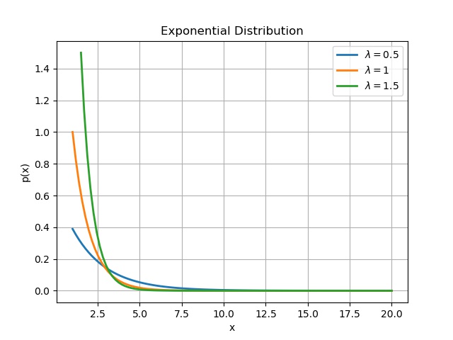
What the historical Python curves plot

The code sets loc=llambda and scale=1./llambda. In SciPy, loc shifts the start of the distribution, so these curves use $f(x)=\lambda e^{-\lambda(x-\mathrm{loc})}$ for $x\ge\mathrm{loc}$, with loc numerically equal to llambda. They are shifted exponential densities, whereas the waiting-time derivation above starts at zero. Their means are loc $+1/\lambda$, and their variances remain $1/\lambda^2$. To plot the unshifted waiting-time density, use loc=0. The first curve is sampled only from 1 onward and omits part of its shifted support, which begins at 0.5. The historical code and its English plot are retained unchanged.

Original Korean learning note