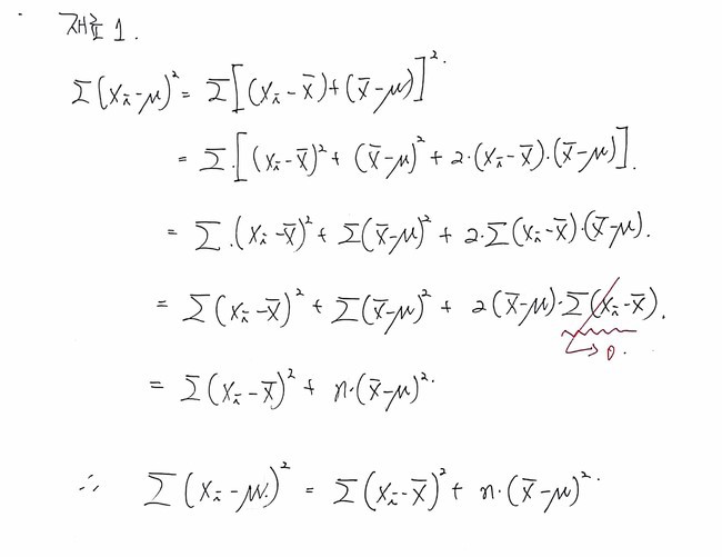
Derivation of the Chi-Squared Distribution

Alright, chi-squared distribution time.

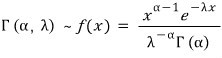
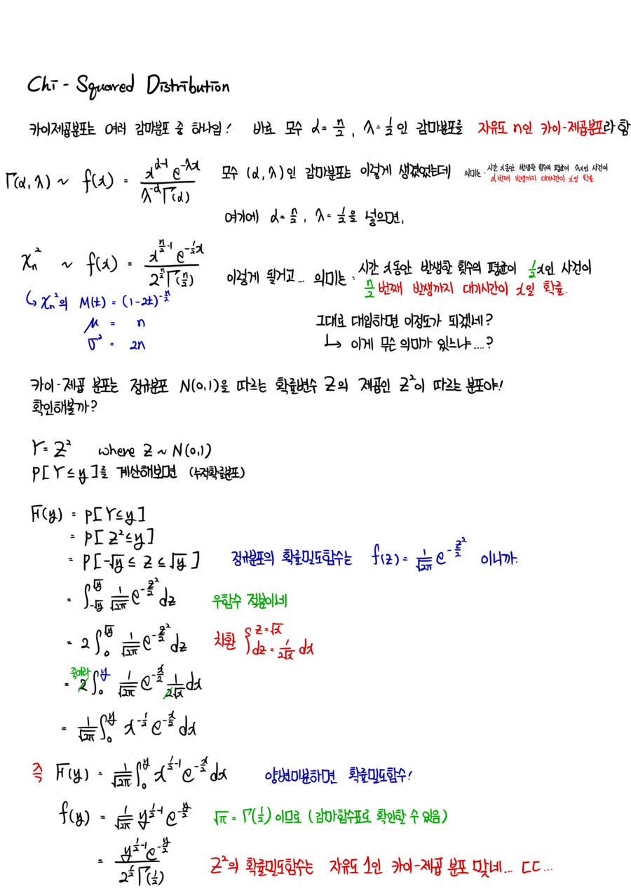
The chi-squared distribution is just one of the gamma distributions $(\alpha, \lambda)$.

Out of all the gammas out there, the one with $\alpha = n/2$ and $\lambda = 1/2$ — that one specifically gets its own name: the chi-squared distribution with $n$ degrees of freedom.

Recall the gamma:

Plug in $\alpha = n/2$, $\lambda = 1/2$ and you get:

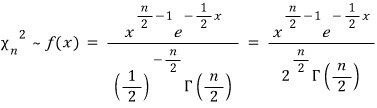
There it is.

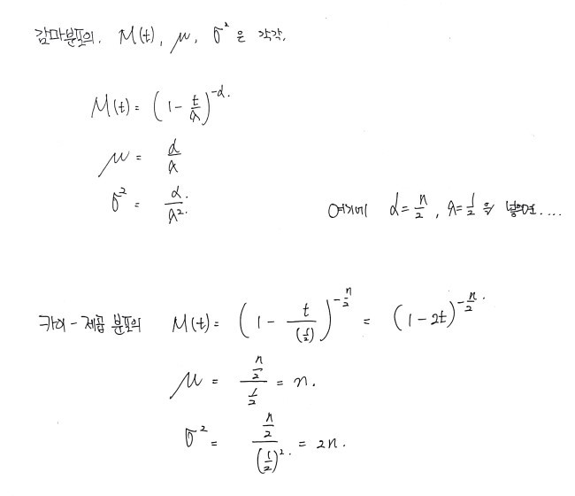
And since this is just a gamma in disguise, the MGF, mean, variance — all of it falls out for free.

So the obvious question: if it’s just a gamma, why bother giving it a separate name? Has to be because it’s a little special, right?

Yeah. It is. And the reason is — it’s tied to the normal distribution.

We usually write the random variable for the normal as $Z$, right? And $Z \sim N(0,1)$.

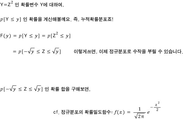
OK but watch this. $Z^2$ follows the chi-squared with 1 degree of freedom. !!!

!!

So given $Z \sim N(0,1)$, let me actually prove that it follows

.

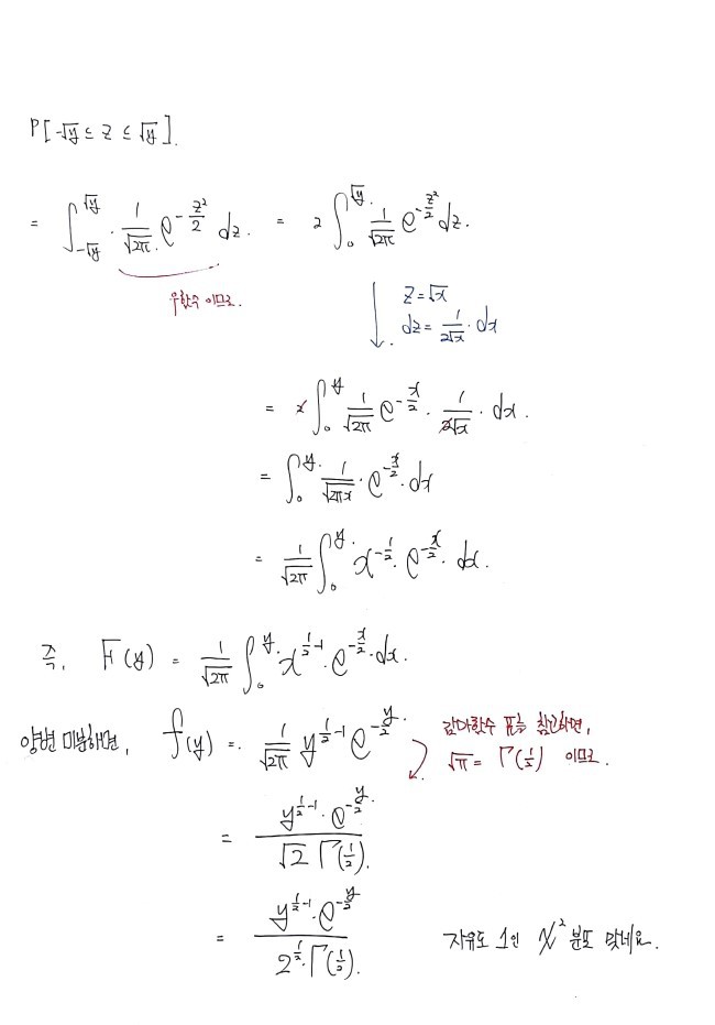
OK. And now that we’ve nailed down that this

follows the chi-squared (which is, again, just a gamma), we get one more thing for free.

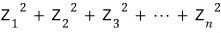
This guy has $n$!!!!!!!!! degrees of freedom — chi-squared, that is.

It follows

!!!!

Why?!?!?! Because the chi-squared is a gamma, and we already worked out the additivity of the gamma distribution in a previous post, remember??~~~~~~~~~~

(Gonna use it like, immediately.)

So I’m gonna skip the proof — go check the previous post, it falls right out. heh

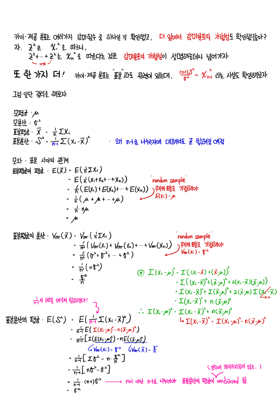
OK, one more thing about the chi-squared and then we’re done.

I said the chi-squared matters because it’s connected to $Z$ from the normal. But actually — it has a deep connection with samples too.

And since that connection is gonna be the bridge over to the $t$-distribution, I figured I should lay it down before we move on.

We already talked about the difference between population and sample waaaaaay~~~~~~ back, but let’s revisit.

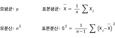
First, just to pin down notation:

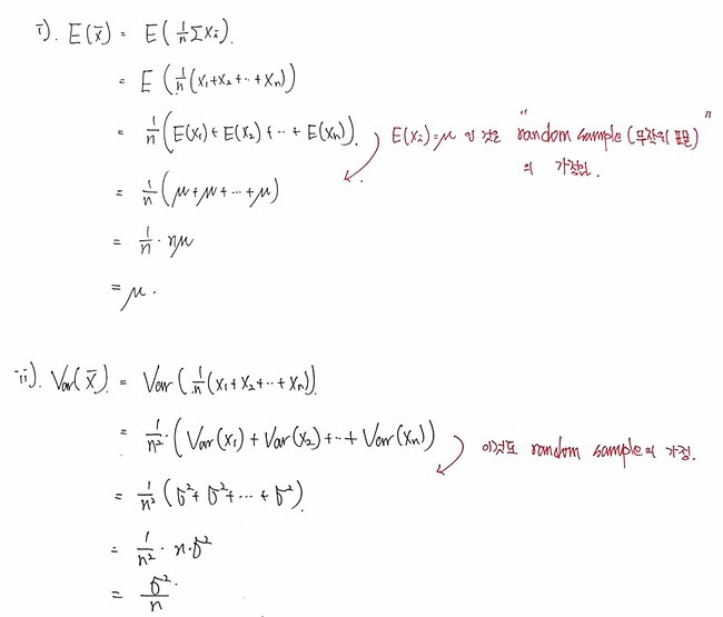
Now that samples are on the table, the population mean and population variance become the things we’re trying to estimate… right…?

Quick aside on that:

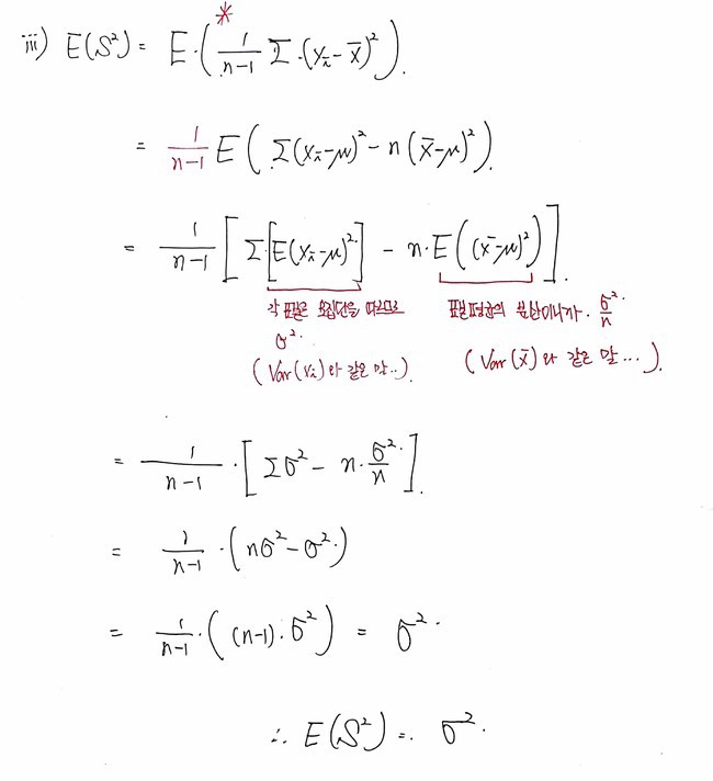
When you compute the sample variance

, you all know we divide by $n-1$ instead of $n$ because we burned one degree of freedom.

But! We also figured this out mathematically!!!!!

The whole point was making the expectation of

unbiased.

(Well… it’s kinda the same thing — it only comes out unbiased if you knock the degrees of freedom down by one… heh)

But that wasn’t actually what we were after right now.

What we want to say is — the chi-squared is connected to

….

OK anyway, back to where we were!!!!!

If the population is Gaussian

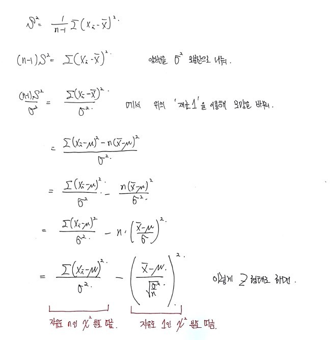
, and we draw a random sample $X_1, X_2, X_3, \dots, X_n$ of size $n$ from it, and define the sample variance as

,

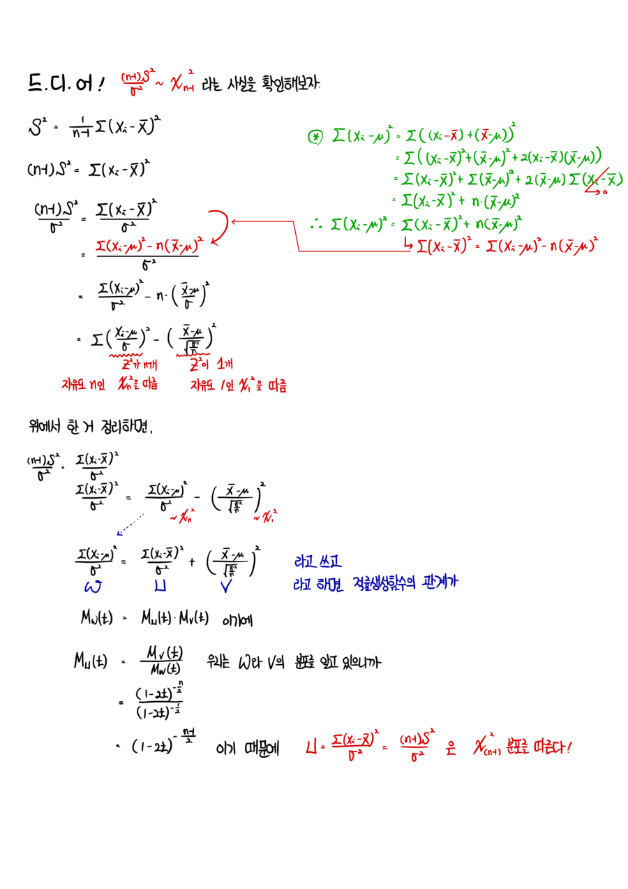
then "

follows the chi-squared with $n-1$ degrees of freedom."

That’s what we wanted to prove!!!!!!!!!!!!!

Let’s gooooooooooo

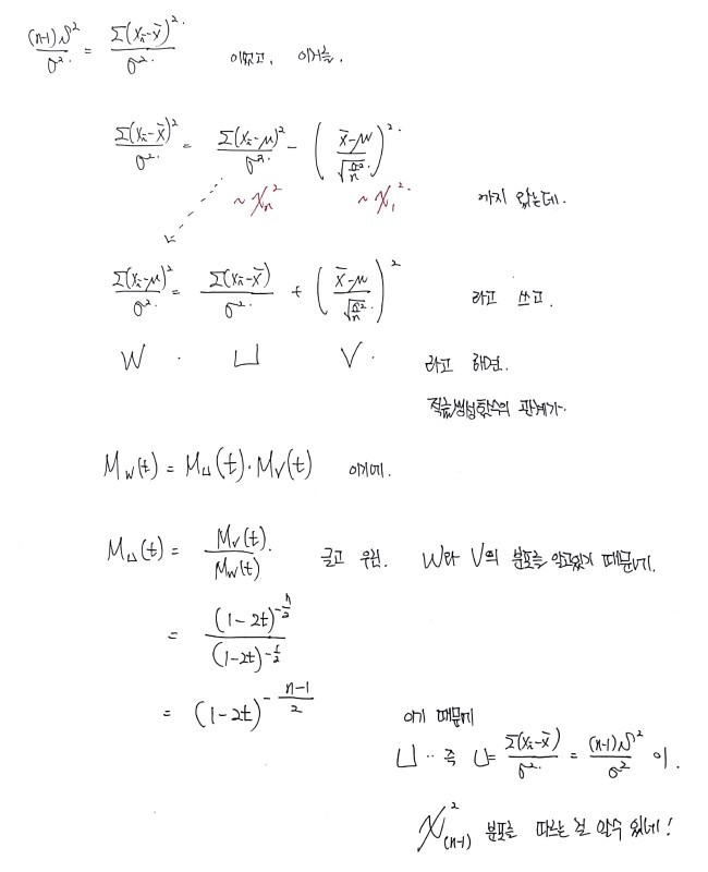
Done~

↓ Cleaned up nicely on the iPad:

P.S.

Did you know?

I converted all my blog posts into PDFs and I’m selling them :-)

https://blog.naver.com/gdpresent/222243102313

Blog Post PDF (ver. 2.0) on sale (Physics I studied, Finance I studied) — purchase info below~ Hi! If there are bits in the blog posts that feel unsatisfying, take a look at the PDFs…

blog.naver.com

1

2

3

4

5

6

7

8

9

10

11

12

13

14

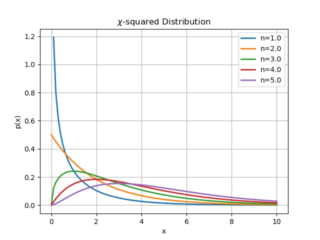
n = [1., 2., 3., 4., 5.]

for i in n:

alpha = i / 2 # i = n

llambda = 0.5

scale= 1./llambda

x = np.linspace(0, 10, 100)

y = sc.gamma.pdf(x, a=alpha, scale=scale)

plt.plot(x, y, linewidth=2.0, label = ‘n=%s’ % i)

plt.grid(True)

plt.legend()

plt.ylabel(‘p(x)’)

plt.xlabel(‘x’)

plt.title(r’$\chi$-squared Distribution’)

plt.savefig(‘4.Chi-squared Distribution.jpeg’)

cs

Originally written in Korean on my Naver blog (2017-11). Translated to English for gdpark.blog.