Derivation of the F-Distribution

This time it’s the F-distribution — the last one in our little parade of distributions.

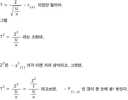
Why study the F-distribution right after the t-distribution? Well, here’s the cute reason: if a statistic $T$ follows the t-distribution, then $T^2$ follows the F-distribution. So they’re basically next of kin.

Buuut that’s not to say the F-distribution is only the distribution that $T^2$ follows —

let’s go more general than that.

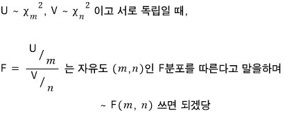
First we need to define the random variable $F$,

and honestly, let me just toss the definition out there first and we’ll talk about it.

where $U$ follows a chi-squared distribution with degrees of freedom

and $V$ follows a chi-squared distribution with degrees of freedom

Since we had

it makes total sense that $T^2$ would follow the F-distribution — I’ll come back and hit this point one more time at the very end.

And while we’re at it, let me throw out the probability density function of the F-distribution too:

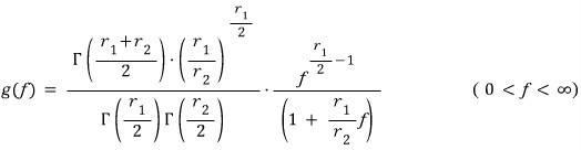
Of course, this whole post is about deriving this F-distribution PDF. So let’s get into it.

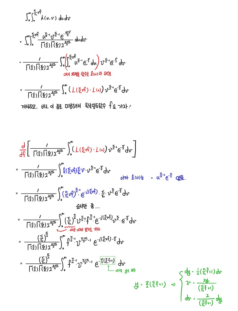
So first up,

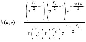
I’m going to construct the joint density function of $U$ and $V$.

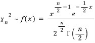
Pulling out the chi-squared PDF as our reference,

I’ll call the joint density of $U$ and $V$ just $h(u,v)$.

(The principle for building this joint density is the exact same one we used in the t-distribution derivation in the previous post.)

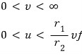
OK, and after that — for the cumulative distribution…

I want to write it as $F(\sim)$, but that’s gonna get super confusing because we already have $F$ doing other work here.

So let me use a different symbol for the CDF in this post!!!

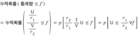
That’ll do, I think.

And from here on, it’s by hand;;;;

Typing this out is way too much~~~~~~~~~~~~~~~~~~~~~~~~~~~~~~~

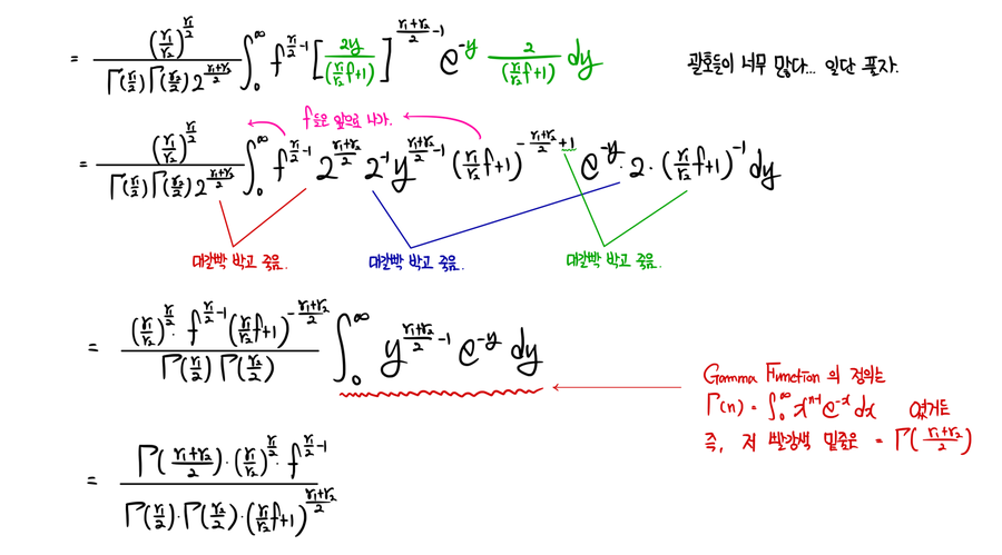
OK so the derivation is done.

Let me grab a few basic properties of the F-distribution and wrap this thing up!!!!

Just like before, there’s an F-distribution table for this guy too,

and let me quickly show how to read it —

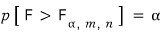
the F-distribution table expresses the $(1-\alpha)$ quantile as

and apparently it means this:

Let me run a quick example with $\alpha = 0.05$~

If you go look it up, you get $5.19$,

and what does that number actually mean?

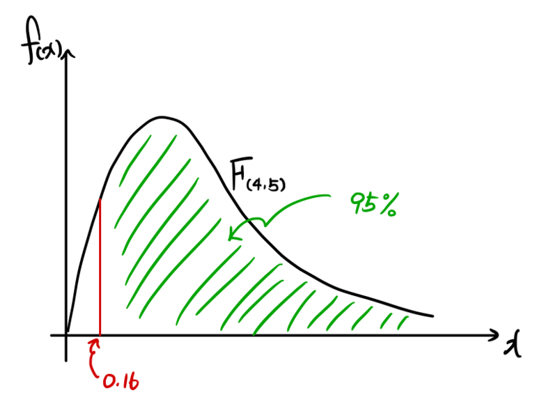
If we draw it as a picture,

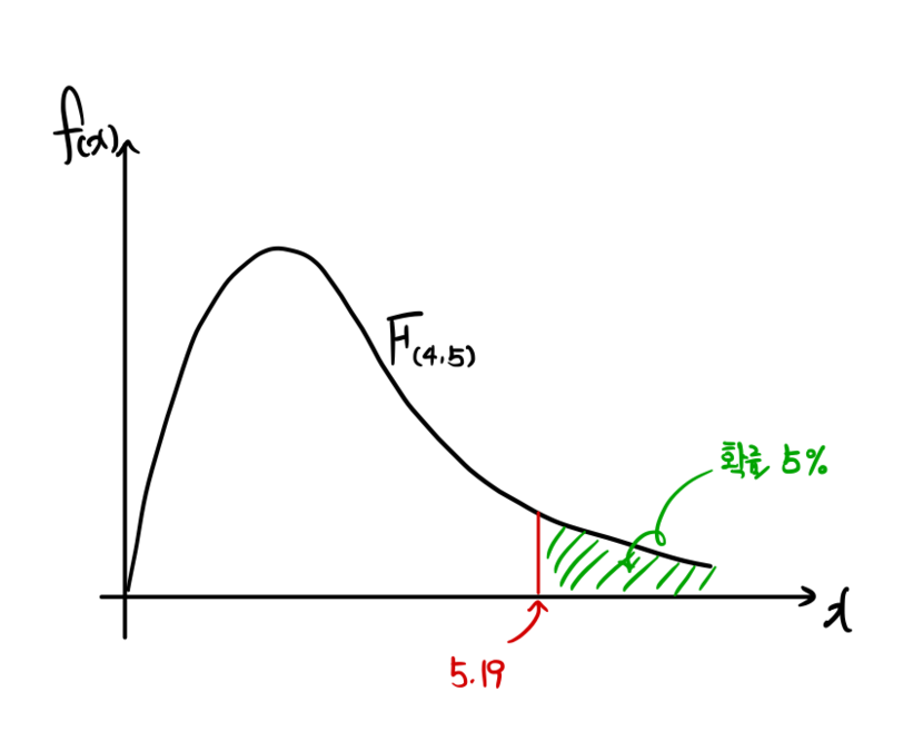
it’d look something like this!

Also also also also also — another property of the F-distribution:

if you swap the numerator and denominator in the definition, you get an F-distribution with the degrees of freedom flipped. So:

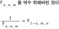
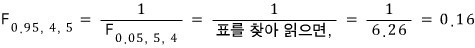
So for instance,

if you want to find

but there’s no table for $\alpha = 0.95$,

even with just the $\alpha = 0.05$ table, you can still get the answer like this!

So that’d be this kind of picture:

Also, summarizing a bit more about the F-distribution,

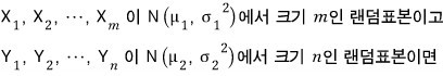
The two random samples have to be independent too!!!!

Then

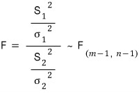
that’s the content,

and the principle is simple.

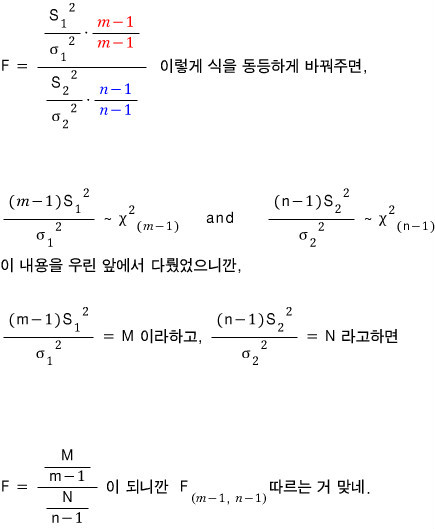
Also, waaay back~~~~~~ at the very beginning,

I said that if $T$ is a statistic that follows the t-distribution,

then $T^2$ follows the F-distribution —

let’s actually verify the degrees of freedom too (of course, everyone’s already finished this calc in their heads by now… (crying))

And that’s just the F-distribution in a nutshell.

Now let’s talk a bit about testing..

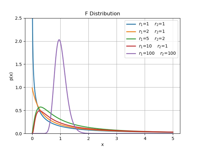
r1 = [1, 2, 5, 10, 100]
r2 = [1, 1, 2, 1, 100]
r = list(zip(r1, r2))
for i, j in r:                   # i = n
    x = np.linspace(0, 5, 1000)
    y = sc.f(i, j).pdf(x)
    plt.plot(x, y, linewidth=2.0, label = r'$r_1$=%s    $r_2$=%s' % (i, j))
plt.grid(True)
plt.legend()
plt.ylabel('p(x)')
plt.xlabel('x')
plt.ylim(0, 2.5)
plt.title('F Distribution')
plt.savefig('8.F Distribution.jpeg')

Originally written in Korean on my Naver blog (2017-11). Translated to English for gdpark.blog.