Hypothesis Testing
A casual walkthrough of hypothesis testing basics — null vs. alternative hypotheses, Z-statistics, and how to decide when to reject what the data's telling you.
Just want to cover some very basic testing stuff and then move on.
So first — what even is hypothesis testing?
“When you’re judging some unknown parameter from observed samples, the act of trying to keep the chance of being wrong about that judgment under a pre-set level.” That’s hypothesis testing.
OK let me just throw out an example.
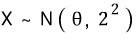
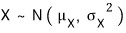
EX. Suppose a certain company’s lightbulbs have a lifespan that follows a normal distribution, and they run quality control so the mean is 1500 hours and the standard deviation is 100 hours.
That is — if you write the lifespan as a random variable X, then X ~ N(1500, 100²).
Now the R&D team at this company comes out and claims they’ve developed a new product — same cost, same standard deviation as the existing one, but the mean lifespan is longer.
To check this, they test-produced 25 of them, measured the mean lifespan, and got:

From this result — can we really be sure the new bulb’s mean lifespan is longer than the existing one’s?
When you’re staring down a question like this,
you do hypothesis testing.
And first — since the R&D folks are claiming the mean lifespan is 1500 hours or more, let’s set up the hypotheses like this:
θ represents the ‘mean lifespan’. Let me explain a bit about hypothesis testing by walking through what H_0 and H_1 are.
These guys’ claim was: “the new bulb’s mean lifespan is longer than the existing one’s mean of 1500.” That claim gets written over there as
This —

— is called the alternative hypothesis.
And this —

written as
— is called the null hypothesis.
The “null” here is the null of nullify — to make invalid.
That is, "

is the hypothesis that nullifies the alternative hypothesis

."
So we set up these two hypotheses, and the act of deciding which one to adopt and which one to reject — that is called ‘hypothesis testing’.
But of course, you’d need to be armed with some basis and logic that shuts everyone up before you can claim “this one’s adopted, that one’s rejected.” There are various criteria for testing, but here we’ll do the example with the Z-statistic.
Because there’s still more basic terminology we need to nail down.
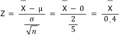
Let’s think about the Z-statistic.
The standard deviation of

is

, so it’s 20.
And under H_0:
and when

is large enough (i.e. when the mean of what we sampled in the trial comes out absurdly large),
that is, when
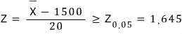
we reject

and adopt the alternative hypothesis

.
Why does
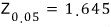
this become the cutoff — well, that’s kind of up to whoever’s doing the test….
But in stats, apparently

or

get used a lot. (More on this later.)
Anyway —
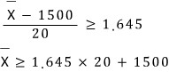
if the mean of our measured sample exceeds that value, we get to reject H_0 and adopt H_1 — that!
What this actually means, deep down, we’ll come back to in a sec!!!
Before that, let’s organize the terminology here.
A statistic that serves as the standard for testing — like the Z-statistic when you’re testing by this kind of criterion — is called the test statistic.
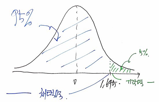
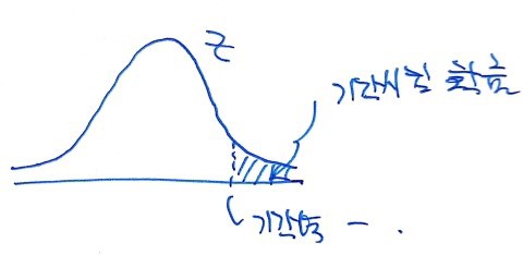
And a region like Z ≥ 1.645, the “region where the null gets rejected,” is called the critical region.
The rest of it — everything else — is called the acceptance region.
(cf. The boundary between them is called the critical point.)
(Whether we phrase it as ‘rejecting’ the null hypothesis or ‘adopting’ the alternative — that’s the standard.)
If we draw the critical region and acceptance region:
Now let’s dig a little more into what Z ≥ 1.645 actually means.
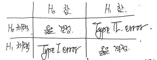
First — in testing, there are two kinds of ’errors’:
When the null hypothesis H_0 is true, but you adopt H_1 anyway: Type 1 error
When the alternative hypothesis H_1 is true, but you adopt H_0 anyway: Type 2 error
So,
we observe sample X̄, look at the Z-statistic from it, and let’s say it lands in the critical region — and I rejected the null.
But —
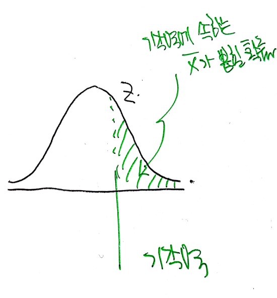
what this graph is telling us is “the probability of being drawn when X̄ is drawn,” right?
That is, “the probability of drawing an X̄ that lands in the critical region when X̄ is drawn” — that green chunk over there in the diagram!!!
So what Z ≥ 1.645 actually means is: “the probability that even though the null hypothesis is true, by sheer chance this particular trial gave us an X̄ big enough that we end up rejecting H_0.”
That is — “the probability of committing a Type 1 error” lives right here:

We say that number means “the permissible limit of the probability of committing the error of rejecting H_0 when H_0 is actually true and adopting H_1 instead.”
It’s called the significance level, and apparently it’s commonly written as α.
So α = 5% means: out of 100 trials, a true hypothesis isn’t rejected more than 4 times… wait, that’s “isn’t rejected” — (I mean, the true hypothesis gets rejected no more than 5 times out of 100).
The confidence level is 95%, and the confidence coefficient is 1 − α — that!
By the way, the significance levels people commonly use are 1%, 5%, and 10%.
OK so — since the R&D team’s sample mean for n = 25 was 1550,
Z = 2.5,
and since Z = 2.5 > 1.645 (it’s in the critical region),
“at significance level 5%” we get to draw the conclusion: reject the null, adopt the alternative.
At this point, let’s look at the p-value.
The mean the team got from their sample was 1550, and the Z-statistic for that was Z = 2.5, right? Then if Z = 2.5,
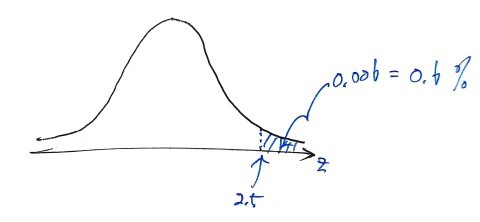
which means: “even if we’d run the test at significance level 0.6%, H_0 would still have been rejected. The only way H_0 wouldn’t have been rejected is if the significance level was set below 0.6%.”….
Right here, that 0.6% — that’s called the p-value (or significance probability), apparently.
The meaning of the p-value is: ’the minimum significance level at which the null hypothesis H_0 can still be rejected for the given test statistic.’
So when X̄ = 1550 vs. when X̄ = 1600, both would lead to rejecting H_0 — but the p-value tells us that the larger X̄ is, the smaller the p-value gets, and the degree of certainty that H_1 is true can be different in each case. That’s what the p-value is capturing.
OK, now those terms that felt totally foreign earlier are starting to feel a little more familiar.
Let me lightly cover the few terms we haven’t hit yet —

A hypothesis like this, where the parameter value is pinned to a single point, is called a simple hypothesis.

A hypothesis like this, where the parameter value is given as a range, is called a composite hypothesis… ;;; just terminology ;;;
But apparently, in general, the null hypothesis is written as a simple hypothesis and the alternative as a composite hypothesis.
Power function
- In any given test method, the function that expresses “the probability of rejecting H_0” (i.e. the probability of landing in the critical region) as a function of the parameter θ is called the power function,
and mathematically it’s written as
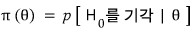
!!
- The value of the power function at a specific θ belonging to the alternative hypothesis H_1 is called the power, apparently.
Let’s say
. And when we use a sample of n = 25,
let’s say

follows the standard normal distribution, and if we calculate π(θ) for a given θ:
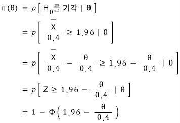
(Here uppercase Φ is the ‘cumulative probability’, riiight?)
And then if we keep cranking out π(θ) for θ = 0, θ = 0.4, θ = 1, etc. etc. etc., we get a bunch of values.
These values get produced…
and what you get when you plot them on a graph — that is the power function.
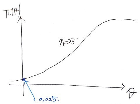
Let me focus on just that one marked point.
It’s been set so that the function value at θ = 0 in π(θ) is 0.025.
This means: the probability of rejecting the null when θ = 0.
And the probability of rejection is
since this means the probability right here —
we’ve seen this somewhere before, haven’t we?!?!?!?
It was the diagram about the significance level, wasn’t it???
That is — the function value of π(θ) for each θ in the power function
turns out to be the α value!!! Which is just a synonym for “the probability of committing a Type 1 error!”
Now let’s look at this with the t-statistic.
(And while we’re at it — earlier we only did one-tailed examples, so let’s look at what two-tailed means at the same time.)
As we saw, when X follows
,
then it follows
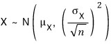
,
so
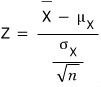
follows the standard normal distribution, which is nice —
but usually

is unknown. That’s the trap.
So let’s say we replaced that

with

.
That is —

we’ve replaced it with this.
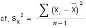
Now this guy no longer follows a normal distribution — as we saw earlier, you have to treat it as a t-distribution with n − 1 degrees of freedom.
So this time, let’s look at the 95% confidence interval and the critical t-value at that point using the T-statistic!
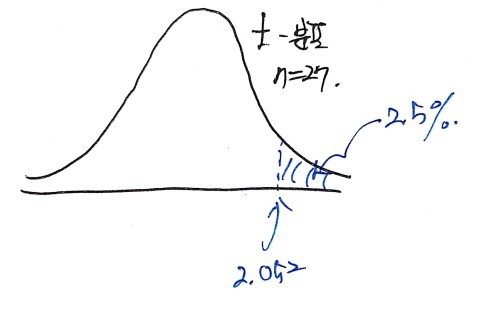
With a “two-tailed test”!!! (Degrees of freedom: 27. So sample size is 28.)
Looking up the t-distribution table,
we can confirm:
!
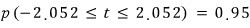
That is — when df = 27, the probability that the observed t-value falls in (−2.052, 2.052) is 95%, and here −2.052 and 2.052 are called the critical t-values.
t = −2.052 is the lower critical t-value, and the other one is the upper critical t-value.
And now, if we change

into
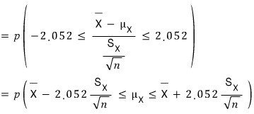
, this means the probability that μ_X lives inside this interval is 95%.
That is — when μ_X is observed, we can expect 95 out of 100 times it’ll land inside that interval. The significance level is 5%, or equivalently the probability of a Type 1 error is 5%… same thing as before.
This time, let me throw out a quick example of testing via the chi-squared distribution before I head out.
Chi-squared testing is usually what you do when S is known but you’re testing an unknown σ. The basic principle is the same as the testing we’ve already done, so it shouldn’t be that bad.
Say S² for 31 observations from a normal-distribution population is 12.
And let’s set up

.
Then the

statistic follows the

distribution.
And if we set α = 5%, the confidence interval looks like this:
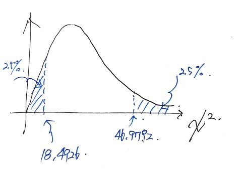
But if σ² is 9,
since
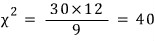
, it lands in the acceptance region in the graph above.
So the conclusion is: “we do not reject the null hypothesis.”
That was a surface-level look at testing.
After this, in a ‘statistics’ post rather than a ‘statistics basics’ post, I’ll deal with more and more detailed problems.
Originally written in Korean on my Naver blog (2017-11). Translated to English for gdpark.blog.
Comments
Discussion happens via GitHub Discussions. You'll need a GitHub account to comment.