Temperature [Thermal & Statistical Mechanics I Studied #4]

Original Korean learning note

Translation of the complete original note. Historical source statements and errors are preserved; eight separate editorial clarifications follow.

The statistical definition of temperature

Finally, the book is going to look at what this thing called ’temperature’ is!!!

After thinking about the definition of temperature,

the conclusion I finally arrived at is downright staggering!!!! So let’s get started!

First, let me set things up.

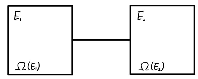
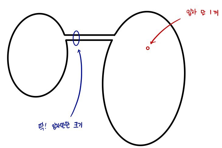
I’ll place two systems,

and those two systems can exchange energy with each other,

but I’ll say they don’t exchange energy with any other system.

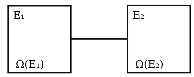
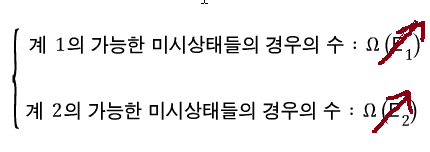
Two similar rectangular systems joined by a horizontal line. The left has E1 and Omega(E1); the right has E2 and Omega(E2).

The left-hand system (number 1) contains energy $E_1$ and what I’ve written as $\Omega$ means a ’number of possibilities.'

Which possibilities? The ’number of possible microstates’ that system 1 can have when it has energy $E_1$ .

Alright, so the left-hand system will be in one of $\Omega(E_1)$ microstates.

The right-hand system will be the same.

What about the combined system, then?

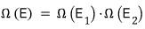
$E=E_1+E_2$ is its energy, so it will be in one of $\Omega(E_1+E_2)$ microstates.

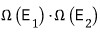
But that number, $\Omega(E_1+E_2)=\Omega(E_1)\Omega(E_2)$

will equal the product of the two counts!!!!

$\Omega(E_1)\Omega(E_2)$ is the number of states, and I’ll say it is in one of them.

Now we make a few assumptions.

(The flavor of these assumptions is something like, “It sounds plausible, so let’s assume things work this way!”)

All possible microstates are equally likely to occur.

(That means treating each event as an elementary event, right?)

The movement of ‘something’ inside a system continually changes that system’s microstate.

In other words, the internal microstate keeps on changing.

(Copied from the text) Given enough time, the system will explore all its possible microstates and spend equal amounts of time in each of them. (The ergodic hypothesis)

* To flesh out the ergodic hypothesis just a little,

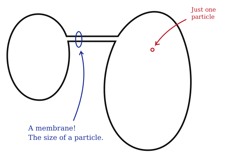
Blue: “A membrane! The size of a particle.” The curved blue arrow points up to the membrane at the connecting neck. Red: “Just one particle.” The red arrow points to the sole particle in the right chamber.

The particle in that right-hand container will keep moving,

and it is connected to the left-hand system. (That means they can exchange energy.)

Now, as the particle moves, can we really say it will eventually cross over into the left-hand system?

No. No!!!!

Apparently, a situation like this is called ’nonergodic.’

Anyway, from those three assumptions, our conclusion is

“This system selects a single macroscopic arrangement that maximizes the number of microstates.”

The book explains it as above, but here’s how I think about it.

First, we cannot distinguish individual microstates.

But we can distinguish macrostates.

In other words, when we open the lid, we can say, “Aha, it changes like this: this macrostate, that macrostate, and so on!”

We can’t distinguish changes in microstates at all, and they don’t mean anything to us~.~

So even though the system is changing, we should say that, to our eyes, it is likely to be in the macrostate that contains the largest number of microstates.

When the system is small, that is all we can say…

But when the system is large, apparently we can say, “The likelihood is ridiculously, overwhelmingly—no, just fucking high.”

In our picture, when energy is exchanged, $E$ allocates energy to $E_1$ and $E_2$.

When it makes that allocation in the large combined system,

we can say that it “allocates energy so that the number of microstates belonging to the same macrostate is as large as possible.”

I forced those arrows into the picture to emphasize that these are ’energy variables,’ rather than constants,

and we should choose those variables so that the number of microstates belonging to the same macrostate is as large as possible.

We will choose the variables that make it a maximum.

Let’s decide using calculus!

$$ \Omega(E)=\Omega(E_1)\Omega(E_2) $$

For a function of $E$ like this, $\Omega(E)$

we just need to find the energy that makes this guy’s function value as large as possible!!!

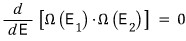
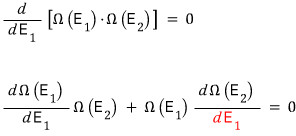
$$ \frac{d}{dE}\bigl[\Omega(E_1)\Omega(E_2)\bigr]=0 $$

It is the same logic as differentiating $f(x)$ with respect to $x$ in high-school calculus to find the maximum of $f(x)$, I guess. (We are looking for an extremum.)

But let’s differentiate with respect to $E_1$. That should be fine, right?

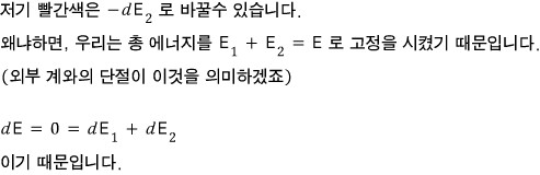
$$ \begin{aligned}\frac{d}{dE_1}\bigl[\Omega(E_1)\Omega(E_2)\bigr]&=0\\[1em]\frac{d\Omega(E_1)}{dE_1}\Omega(E_2)+\Omega(E_1)\frac{d\Omega(E_2)}{\color{#c00020}{dE_1}}&=0\end{aligned} $$

That red part can be replaced with $-dE_2$.

That is because we fixed the total energy at $E_1+E_2=E$.

(The absence of an external system must have meant this.)

$$ dE=0=dE_1+dE_2 $$

That is why.

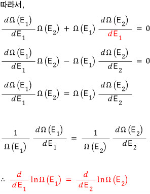
Therefore,

$$ \begin{aligned}\frac{d\Omega(E_1)}{dE_1}\Omega(E_2)+\Omega(E_1)\frac{d\Omega(E_2)}{\color{#c00020}{dE_1}}&=0\\[.5em]\frac{d\Omega(E_1)}{dE_1}\Omega(E_2)-\Omega(E_1)\frac{d\Omega(E_2)}{dE_2}&=0\\[.5em]\frac{d\Omega(E_1)}{dE_1}\Omega(E_2)&=\Omega(E_1)\frac{d\Omega(E_2)}{dE_2}\\[1em]\frac{1}{\Omega(E_1)}\frac{d\Omega(E_1)}{dE_1}&=\frac{1}{\Omega(E_2)}\frac{d\Omega(E_2)}{dE_2}\\[1em]\therefore\quad\color{#c00020}{\frac{d}{dE_1}\ln\Omega(E_1)}&\color{#c00020}{=\frac{d}{dE_2}\ln\Omega(E_2)}\end{aligned} $$

A situation? (A condition?) like the red equation is the condition for an energy allocation that maximizes the macrostate containing the most of the same microstates!

Hah… finally, the conclusion.

At that point, there will be that exact!! Temperature!!!! (Earlier, I said temperature was one of the “macrostates.”)

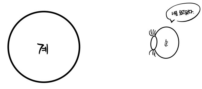
The temperature we measure—the temperature we find when we open the lid!!!—is defined in terms of the energy above.

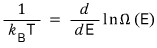
In other words, both sides of that red equation are defined through temperature.

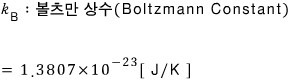
$$ \frac{1}{k_B T}=\frac{d}{dE}\ln\Omega(E) $$

$k_B$: Boltzmann constant

$$ 1.3807\times10^{-23}\ [\mathrm{J/K}] $$

Apparently, the equation above has also been proved experimentally.

In fact,

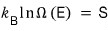
$$ k_B\ln\Omega(E)=S $$

defining this as ’entropy’ was Boltzmann’s achievement.

But for now, let’s just count this as having heard of it once and move on.

Ensemble

I think I need to explain the concept of an ensemble first.

Suppose what we want to know now

is something about a system sitting in front of us.

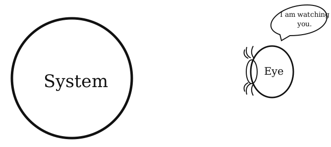
A large system circle on the left faces a smaller stylized eye with eyelashes on the right. The eye has a speech bubble saying I am watching you. — System: the large circle on the left. Eye: the eye on the right. Speech bubble: “I am watching you.”

Say there are 50 million particles in there, and we want to know the average velocity of the particles inside that system.

Alright, we take one measurement and obtain a result called <v>.

“Can you trust it?”

It would feel a bit uneasy, wouldn’t it?

So we want to take a second measurement,

but after that first measurement, the system has been disturbed, so none of the variables are at their initial values…

That makes the result of that experiment even, even, even less trustworthy. (We cannot make the measurement under the same conditions.)

How can we solve this difficult problem?

We click Copy on the initial system and prepare around 2.5 billion identical systems.

Then we have identical systems, right?!!?!? We repeat the experiment 2.5 billion times and collect 2.5 billion average-velocity data points.

If we call the average of these results <v>, doesn’t that sound a little more convincing?

The ensemble is a concept introduced out of this wish.

We put an infinite number of exactly identical systems together.

<Actually, this is the same concept as ‘statistical probability’ in high-school probability and statistics.

When we throw a die and say, “The probability of getting a two is 1/6!!!” …that is actually a funny thing to say.

We would have to throw it infinitely many times or so to reach a probability of 1/6…right?!~>

What we will now find is “the probability that a system is in a particular microstate at a fixed temperature.”

We will use the canonical ensemble to do that.

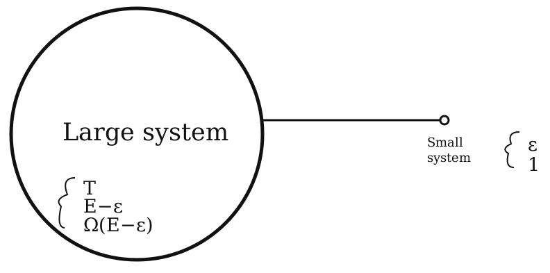
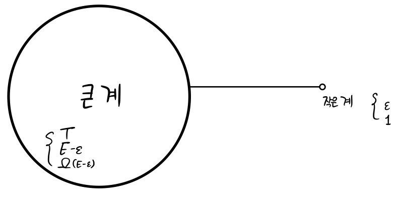
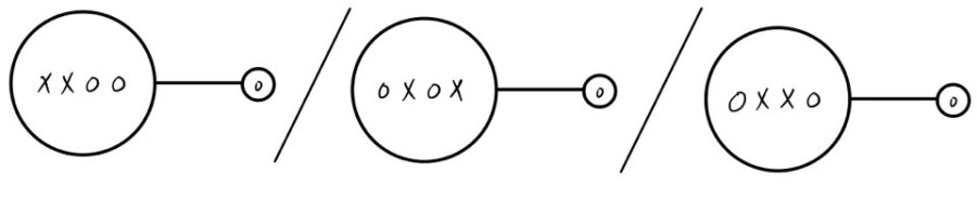
A large bath circle on the left connects by a line to a tiny open circle on the right. The large system has a three-line brace T, E minus epsilon, Omega(E minus epsilon); the small system has a two-line brace epsilon and 1. — Large system: the large circle, with brace entries $T$, $E-\varepsilon$, and $\Omega(E-\varepsilon)$. A horizontal line connects it to the tiny Small system, with brace entries $\varepsilon$ and $1$.

We let a large system like this and a small system exchange energy with each other.

Also, we fix the total energy at $E$, and set the energy of one side to $E-\varepsilon$, this much,

and that of the other side to $\varepsilon$, this much.

And when the large system has energy $E-\varepsilon$, its number of possible microstates is $\Omega(E-\varepsilon)$.

We will assume that the small system has $\Omega(\varepsilon)=1$ possible microstate. (That is how small it is!)

If the number of microstates of the large system that allow the small system to have energy $\varepsilon$ increases,

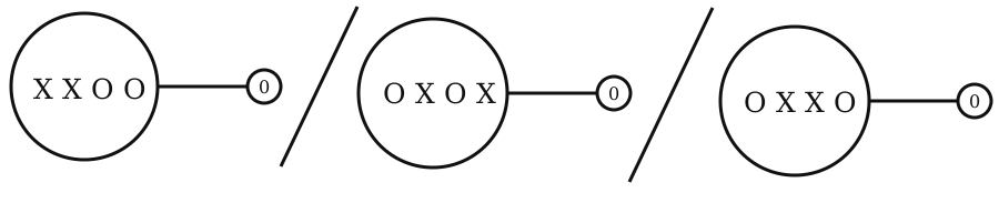
Three large-circle arrangements XXOO, OXOX, and OXXO in order. Each connects horizontally to a tiny circle containing the source mark 0. Two slanted separators distinguish the examples.

as in this picture, the more states in the large system that allow the small system to have energy $\varepsilon$,

the more likely the small system is to have energy $\varepsilon$, so

$$ P(\varepsilon)\propto\Omega(E-\varepsilon) $$

we can write a proportionality like this.

Using the definition of temperature on the right-hand side of this proportionality, we will eventually discuss the Boltzmann distribution.

Let’s keep going.

The large system is really, ridiculously huge,

so $\Omega(E-\varepsilon)$ this is a number, and it is such a huge number that we will take its logarithm and analyze it.

$$ \ln\bigl(\Omega(E-\varepsilon)\bigr) $$

Like this… If we fiddle a little more with the logarithmic expression of $\Omega$, we can connect it to temperature.

And we will Taylor-expand around $\varepsilon=0$. (Apparently, this means “Let’s treat the small system as almost nonexistent!”)

First, let me write down the Taylor expansion.

For $x$ near $a$,

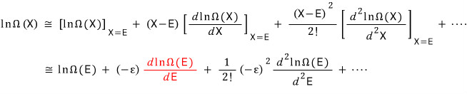
$$ f(x)=f(a)+(x-a)\left.\left(\frac{df}{dx}\right)\right|_{x=a}+\frac{(x-a)^2}{2!}\left.\left(\frac{d^2f}{dx^2}\right)\right|_{x=a}+\cdots $$

We apply this directly to $\ln\bigl(\Omega(E-\varepsilon)\bigr)$ around $\varepsilon=0$, so

I’ll just think of it like this.

Set $E-\varepsilon=X$.

You can think of this as $X\approx E$, too!

$$ \begin{aligned}\ln\Omega(X)&\cong\left[\ln\Omega(X)\right]_{X=E}+(X-E)\left[\frac{d\ln\Omega(X)}{dX}\right]_{X=E}+\frac{(X-E)^2}{2!}\left[\frac{d^2\ln\Omega(X)}{d^2X}\right]_{X=E}+\cdots\\[1em]&\cong\ln\Omega(E)+(-\varepsilon){\color{#c00020}\frac{d\ln\Omega(E)}{dE}}+\frac{1}{2!}(-\varepsilon)^2\frac{d^2\ln\Omega(E)}{d^2E}+\cdots\end{aligned} $$

We will rewrite the red part using the statistical definition of temperature.

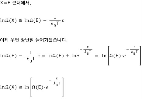
Near $X=E$,

$$ \ln\Omega(X)\cong\ln\Omega(E)-\frac{1}{k_B T}\varepsilon $$

Now, let me play around with this for a bit.

$$ \ln\Omega(E)-\frac{1}{k_B T}\varepsilon=\ln\Omega(E)+\ln e^{-\frac{\varepsilon}{k_B T}}=\ln\left[\Omega(E)\cdot e^{-\frac{\varepsilon}{k_B T}}\right] $$$$ \ln\Omega(X)\cong\ln\left[\Omega(E)\cdot e^{-\frac{\varepsilon}{k_B T}}\right] $$

I will change the symbols and write the same thing again.

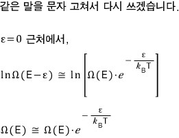
Near $\varepsilon=0$,

$$ \ln\Omega(E-\varepsilon)\cong\ln\left[\Omega(E)\cdot e^{-\frac{\varepsilon}{k_B T}}\right] $$$$ \Omega(E)\cong\Omega(E)\cdot e^{-\frac{\varepsilon}{k_B T}} $$

Earlier, we wrote the proportionality for the probability that the small system has energy $\varepsilon$ as

$$ P(\varepsilon)\propto\Omega(E-\varepsilon) $$

and if we rewrite the right-hand side using the approximation,

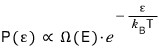
$$ P(\varepsilon)\propto\Omega(E)\cdot e^{-\frac{\varepsilon}{k_B T}} $$

The important thing is that $P(\varepsilon)$ is proportional to that exponential term.

Written like this,

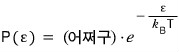
$$ P(\varepsilon)=(\text{something})\cdot e^{-\frac{\varepsilon}{k_B T}} $$

what I want to say is that “The probability $P(\varepsilon)$ that the small system has energy $\varepsilon$ has this probability distribution”!!!!!

So we call this the Boltzmann distribution, or the canonical distribution (literally, “proper-framework distribution”),

$e^{-\frac{\varepsilon}{k_B T}}$ and call this the Boltzmann factor!!!!

It also means that when systems are put in contact, they move toward equilibrium at that temperature $T$!!!

Toward the macrostate with the most microstates…

You still don’t know what this means, right!!!!! I don’t really understand what it means yet either.

Once we work through some problems later, you will probably get a rough feel for it.

You are probably having a mental meltdown right now, so I’ll toss in just one more concept!!!! Hahahahahaha.

This is probability right now, probability!

For it to properly mean a probability, we need normalization.

Making “the sum of all probabilities equal to 1” is what we call normalization, right?!?!?!

$$ P(\text{any microstate})=\frac{P(\text{any microstate})}{\sum P(\text{possible microstates})} $$

Apparently, they normalize using this method here.

Now, let’s rewrite the denominator using the Boltzmann distribution we learned above.

(We have to assume that the system follows the Boltzmann distribution, right!?)

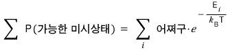
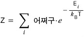
$$ \sum P(\text{possible microstates})=\sum_i (\text{something})\cdot e^{-\frac{E_i}{k_B T}} $$ $$ Z=\sum_i (\text{something})\cdot e^{-\frac{E_i}{k_B T}} $$

This $Z$ is called the partition function.

I have thought about this in my own way,

and I need to record that thought.

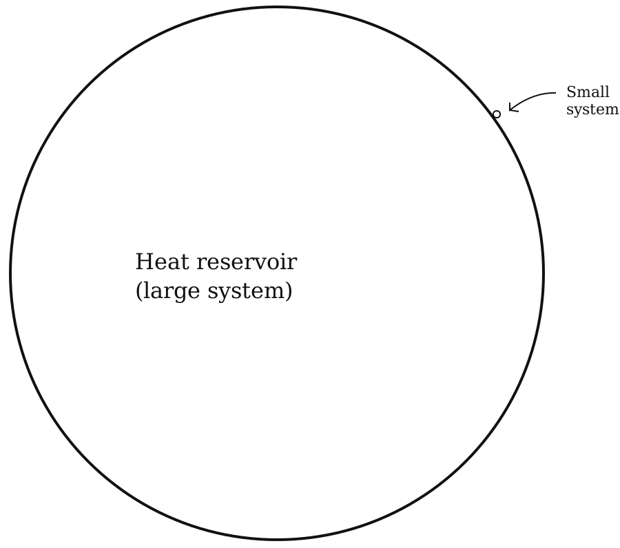
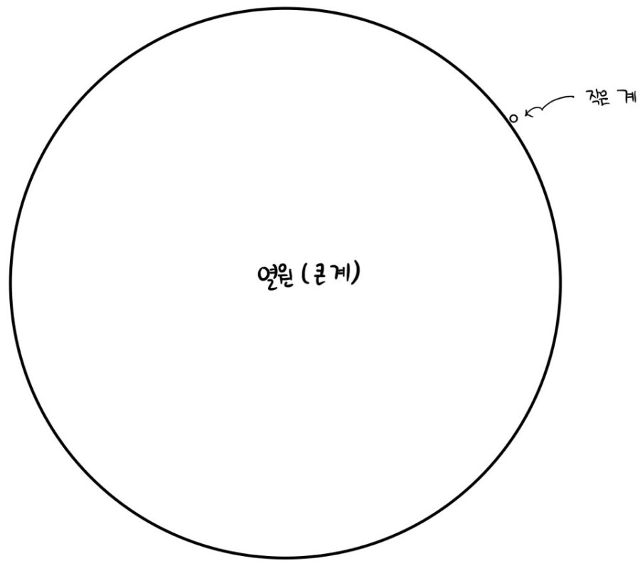
Heat reservoir (large system): the huge circle. Small system: the tiny separate circle just outside its upper-right boundary, indicated by the curved label arrow.

Let us think of a heat reservoir with temperature $T$ and energy $E$.

I drew the picture above in a more extreme way.

When we treated the small system’s energy as $\varepsilon\sim0$, we casually said, ‘Let’s treat the small system as absent in the first place~,’ right?

So, after thinking carefully again about the equation we pulled out with the Taylor expansion,

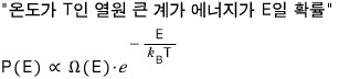
“The probability that a large system at temperature $T$ has energy $E$”

$$ P(E)\propto\Omega(E)\cdot e^{-\frac{E}{k_B T}} $$

I think it was probably saying this.

That is, if the temperature is exactly!! $T$, the energy does not have to be exactly!!! $E$; there is only a probability.

I think that is what it is saying.

This is my own thought, and I have not received advice about it from anyone,

so I am being very cautious. Shoot your arrows at me!!

Until it is proved that I am wrong,

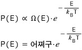
$$ \begin{aligned}P(E)&\propto\Omega(E)\cdot e^{-\frac{E}{k_B T}}\\[1em]P(E)&=\text{something}\cdot e^{-\frac{E}{k_B T}}\end{aligned} $$

I will interpret this as the probability that a system at temperature $T$ has energy $E$, and continue the discussion!!!

In the next post, we will work through some problems from Chapter 4 before moving on.

Separate editorial clarifications

These clarifications are additions to the translation, not statements from the historical note.

For weakly coupled systems at fixed total energy $E$, the count for a specified split is $W(E_1)=\Omega_1(E_1)\Omega_2(E-E_1)$. The complete multiplicity sums or integrates this count over allowed splits. Extremize $W$ or its logarithm with respect to $E_1$, holding $E$ fixed. A vanishing derivative is a stationary condition; a maximum also needs a stability check. At an interior equilibrium maximum, $\partial\ln\Omega_1/\partial E_1=\partial\ln\Omega_2/\partial E_2$. The source product, total-count notation and initial $d/dE$ are retained above; they should not be read as an unrestricted total-count formula.

2. Ergodicity and the membrane illustration

Ergodicity concerns the phase space accessible under the system’s conserved quantities and boundary conditions. If the depicted membrane prevents particle transfer, crossing states are excluded by that constraint. The picture alone does not prove nonergodicity within the accessible region. The translated source’s nonergodic claim remains its historical claim; no permeability assumption has been inserted into the diagram.

3. Equiprobability and macrostate dominance

Equal a priori probabilities apply to accessible microstates under specified microcanonical constraints. A macrostate containing more of these states is more probable, rather than deterministically selected. Fluctuations remain in finite systems. Overwhelming dominance in ordinary macroscopic equilibrium systems is an approximation under the stated ensemble assumptions. Counting alone does not establish a relaxation time or prove that equilibrium will be reached.

4. Temperature, entropy and the constant

In this equilibrium counting framework, $S=k_B\ln\Omega$ and $1/T=(\partial S/\partial E)_{V,N,\ldots}$, with the relevant external parameters fixed. Thus $1/(k_B T)=\partial\ln\Omega/\partial E$. Temperature is a state variable, rather than a complete macrostate. The source rounded constant is retained; the modern SI Boltzmann constant is exactly $1.380649\times10^{-23}\,\mathrm{J/K}$. The temperature relation belongs to an equilibrium framework, rather than an unrestricted experimental proof for every system. NIST: Meet the Constants.

5. Ensembles and measurement

An ensemble is a probability distribution over microscopic realizations compatible with specified macroscopic constraints, rather than a set of exact microscopic clones. An ensemble average differs from a finite sample estimate. A change of microstate alone does not make successive measurements less trustworthy; reproducible preparation and correlations matter. For independent fair-die trials, the probability of two is 1/6 on every trial. Empirical frequency approaches that value as the sample grows; infinite throws are not required for the probability to exist.

6. The subsystem, bath approximation and Taylor notation

For a particular subsystem microstate $i$, $p_i\propto\Omega_{\mathrm{bath}}(E_{\mathrm{total}}-E_i)$. For an energy category, the subsystem degeneracy also enters: $P(\varepsilon)\propto g_S(\varepsilon)\Omega_{\mathrm{bath}}(E_{\mathrm{total}}-\varepsilon)$. The assumption $\Omega(\varepsilon)=1$ is additional; small geometric size alone does not establish it. Keeping the first-order bath expansion requires negligible bath-temperature change over relevant energy exchanges, rather than removing the subsystem or requiring zero absolute subsystem energy. For a stable positive-heat-capacity bath at fixed constraints, the next quadratic correction is $-\varepsilon^2/(2k_B T^2 C_{\mathrm{bath}})$. The Taylor equations above preserve the source factor $(-\varepsilon)^2$ and its printed denominators $d^2X$ and $d^2E$. The intended conventional derivative denominators are $dX^2$ and $dE^2$, respectively; that is a correction to the source notation, not a silent transcription change. The final exponentiated line in the source also prints $\Omega(E)$ on the left, omitting $-\varepsilon$ relative to its preceding logarithmic line. That source typo is retained above. The intended first-order bath relation is $\Omega(E-\varepsilon)\simeq\Omega(E)e^{-\varepsilon/(k_B T)}$; this correction belongs to the separate clarification, rather than to the historical source equation.

7. Normalization and the partition function

Distinguish positive unnormalized weights $q_i$ from probabilities $p_i=q_i/\sum_j q_j$. For discrete canonical microstates, $q_i=e^{-\beta E_i}$ and the standard partition function is $Z=\sum_i e^{-\beta E_i}$, with $\beta=1/(k_B T)$. Summing by energy levels requires degeneracy factors. A common state-independent prefactor cancels from probabilities; a sum including it is a rescaled normalization constant, which cannot automatically replace the standard $Z$ in thermodynamic formulas. The repeated $P$ and the source coefficient “something” are preserved in the translated equations.

8. The speculative closing interpretation

For a system in canonical equilibrium with a larger bath at temperature $T$, its energy can fluctuate and $P_S(U)\propto\Omega_S(U)e^{-U/(k_B T)}$. A particular microstate has the Boltzmann weight; an energy category also has its degeneracy. The combined system remains at fixed total energy, with complementary bath and subsystem energies. Renaming $E$ and $\varepsilon$ does not remove that distinction. The source bare-exponential equality for $P(E)$ omits energy-dependent degeneracy unless an additional special assumption is made. The closing interpretation above remains the author's explicitly tentative interpretation.

The equilibrium counting and canonical-ensemble framework in these clarifications is supported by MIT statistical mechanics notes and MIT canonical-ensemble notes. The boundary-condition, probability and normalization distinctions are separate editorial reasoning.

Original source image archive

Unmodified native image occurrences, retained in original order. The English reconstructions above preserve their substantive content.