Chapter 4 Practice Problems [Thermal & Statistical Mechanics I Studied #5]

Original Korean learning note

Translation of the complete original note. Historical source statements and errors are preserved; eight separate editorial clarifications follow.

I think working through problems is absolutely essential to get a grip on the concepts!

Example 4.3: A two-state system

A two-state system: there are only two states.

One has energy $0$, and the other has energy $\varepsilon\ (>0)$.

What is the expectation value of this system’s energy?

Earlier, we described “the probability that an object at temperature $T$ has energy $\varepsilon$” as

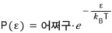
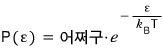
$P(\varepsilon)=\text{blah-blah}\cdot e^{-\frac{\varepsilon}{k_BT}}$ , we said.

That is, the two states here are

(at temperature $T$) the probability of having energy $0$

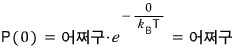
$$ P(0)=\text{blah-blah}\cdot e^{-\frac{0}{k_BT}}=\text{blah-blah} $$

(at temperature $T$) the probability of having energy $\varepsilon$

$$ P(\varepsilon)=\text{blah-blah}\cdot e^{-\frac{\varepsilon}{k_BT}} $$

We also have to do the normalization.

We can just do it like in quantum mechanics, I guess.

$$ \begin{aligned}1&=\text{total probability}=P(0)+P(\varepsilon)\\&=\text{blah-blah}+\text{blah-blah}\cdot e^{-\frac{\varepsilon}{k_BT}}\\&=\text{blah-blah}\left(1+e^{-\frac{\varepsilon}{k_BT}}\right)\end{aligned} $$

Ugh, this doesn’t work…..

This method doesn’t cut it.

So we’ll do the normalization like this

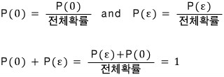
$$ \begin{gathered}P(0)=\frac{P(0)}{\text{total probability}}\quad\text{and}\quad P(\varepsilon)=\frac{P(\varepsilon)}{\text{total probability}}\\[1em]P(0)+P(\varepsilon)=\frac{P(\varepsilon)+P(0)}{\text{total probability}}=1\end{gathered} $$

Let’s build it out.

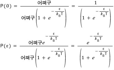
$$ \begin{aligned}P(0)&=\frac{\text{blah-blah}}{\text{blah-blah}\left(1+e^{-\frac{\varepsilon}{k_BT}}\right)}=\frac{1}{1+e^{-\frac{\varepsilon}{k_BT}}}\\[1em]P(\varepsilon)&=\frac{\text{blah-blah}\,e^{-\frac{\varepsilon}{k_BT}}}{\text{blah-blah}\left(1+e^{-\frac{\varepsilon}{k_BT}}\right)}=\frac{e^{-\frac{\varepsilon}{k_BT}}}{1+e^{-\frac{\varepsilon}{k_BT}}}\end{aligned} $$

By expressing the probabilities as a partition function like this, normalization is done, and we can also compute the average.

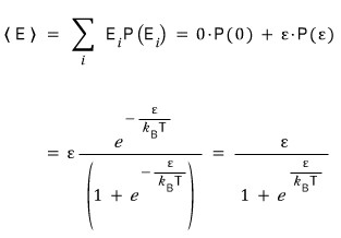
$$ \begin{aligned}\langle E\rangle&=\sum_i E_iP(E_i)=0\cdot P(0)+\varepsilon\cdot P(\varepsilon)\\[1em]&=\varepsilon\frac{e^{-\frac{\varepsilon}{k_BT}}}{1+e^{-\frac{\varepsilon}{k_BT}}}=\frac{\varepsilon}{1+e^{\frac{\varepsilon}{k_BT}}}\end{aligned} $$

Problem 4.2

For the two-state system described in Example 4.3,

derive an expression for the variance of the energy.

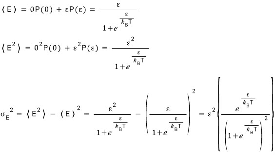
$$ \begin{aligned}\langle E\rangle&=0P(0)+\varepsilon P(\varepsilon)=\frac{\varepsilon}{1+e^{\frac{\varepsilon}{k_BT}}}\\[1em]\langle E^2\rangle&=0^2P(0)+\varepsilon^2P(\varepsilon)=\frac{\varepsilon^2}{1+e^{\frac{\varepsilon}{k_BT}}}\\[1em]\sigma_E^2&=\langle E^2\rangle-\langle E\rangle^2\\&=\frac{\varepsilon^2}{1+e^{\frac{\varepsilon}{k_BT}}}-\left(\frac{\varepsilon}{1+e^{\frac{\varepsilon}{k_BT}}}\right)^2\\&=\varepsilon^2\left\{\frac{e^{\frac{\varepsilon}{k_BT}}}{\left(1+e^{\frac{\varepsilon}{k_BT}}\right)^2}\right\}\end{aligned} $$

Example 4.4: Isothermal atmosphere (air)

Roughly estimate the number of molecules in an isothermal atmosphere as a function of height.

For a system at temperature $T$, the probability of having energy $E$ is

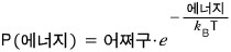
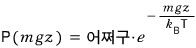
$$ P(\text{energy})=\text{blah-blah}\cdot e^{-\frac{\text{energy}}{k_BT}} $$

Let’s assume there is one gas molecule. And let’s say its energy here is only the potential energy $mgz$.

$$ P(mgz)=\text{blah-blah}\cdot e^{-\frac{mgz}{k_BT}} $$ $$ \text{probability of being at height }z=\text{blah-blah}\cdot e^{-\frac{mgz}{k_BT}} $$

Now let’s say there are many molecules.

Time to cancel the subscription on our “one molecule” assumption, go, go!

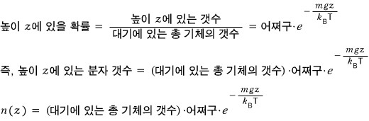
$$ \begin{aligned}\text{probability of being at height }z&=\frac{\text{number at height }z}{\text{total number of gas molecules in the atmosphere}}\\&=\text{blah-blah}\cdot e^{-\frac{mgz}{k_BT}}\end{aligned} $$$$ \begin{aligned}\text{That is, number of molecules at height }z\\=\bigl(\text{total number of gas molecules in the atmosphere}\bigr)\cdot\text{blah-blah}\cdot e^{-\frac{mgz}{k_BT}}\end{aligned} $$$$ n(z)=\bigl(\text{total number of gas molecules in the atmosphere}\bigr)\cdot\text{blah-blah}\cdot e^{-\frac{mgz}{k_BT}} $$

If we plug in $z=0$, it should equal $n(0)$.

So I’ll rewrite the constant like this!!!

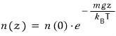
$$ n(z)=n(0)\cdot e^{-\frac{mgz}{k_BT}} $$

Done.

The higher you go, at the rate of the Boltzmann factor $e^{-\frac{z}{k_BT}}$ , it drops off—whoosh~~~ it drops off~—that is what this says.

(Actually, since the real atmosphere isn’t isothermal, they say it’s a bit different, and it’s covered in detail in Chapter 12!)

Problem 4.3

A certain system consists of $N$ states, and each state has energy $0$ or $\Delta$.

Show that the number of arrangements $\Omega(E)$ such that the whole system has energy $E=r\Delta$ ($r$ is an integer) is given by the following expression.

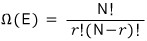
$$ \Omega(E)=\frac{N!}{r!(N-r)!} $$

Each of the $N$ has either $0$ or $\Delta$, and the total energy being $r\Delta$ must mean that $r$ of them are in the energy-$\Delta$ state.

That is, the number of ways of choosing $r$ out of $N$ is the number of possible microstates for $E=r\Delta$!

$$ \Omega(r\Delta)={}_NC_r=\frac{N!}{r!(N-r)!} $$

From this system, remove a small energy $s\Delta$. (The relation $s\ll r$ is satisfied.)

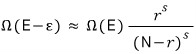
$\Omega(E-\varepsilon)\approx\Omega(E)\frac{r^s}{(N-r)^s}$ —show this.

$\Omega(E-\varepsilon)$ means that out of $N$, $(r-s)$ are in the energy state $\Delta$.

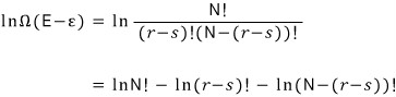
That is, $\Omega(E-\varepsilon)={}_NC_{r-s}=\frac{N!}{(r-s)!(N-(r-s))!}$

$\Omega(E-\varepsilon)$ needs an approximate expression, so we’ll use Stirling’s approximation.

Taking $\ln$ of both sides first,

$$ \begin{aligned}\ln\Omega(E-\varepsilon)&=\ln\frac{N!}{(r-s)!(N-(r-s))!}\\&=\ln N!-\ln(r-s)!-\ln(N-(r-s))!\end{aligned} $$

Now let’s approximate the right-hand side.

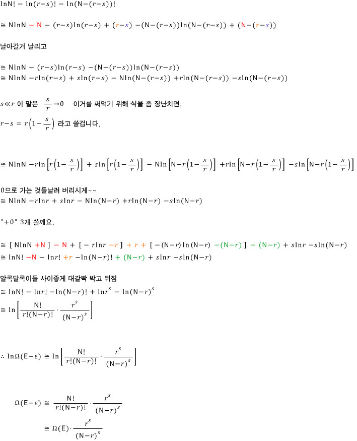
$$ \ln N!-\ln(r-s)!-\ln(N-(r-s))! $$$$ \begin{aligned}\cong{}&N\ln N\textcolor{red}{-N}-(r-s)\ln(r-s)+(\textcolor{orange}{r}-\textcolor{blue}{s})\\&-(N-(r-s))\ln(N-(r-s))+(\textcolor{red}{N}-(\textcolor{orange}{r}-\textcolor{blue}{s}))\end{aligned} $$

Drop the things that will cancel out.

$$ \begin{aligned}\cong{}&N\ln N-(r-s)\ln(r-s)-(N-(r-s))\ln(N-(r-s))\\\cong{}&N\ln N-r\ln(r-s)+s\ln(r-s)\\&-N\ln(N-(r-s))+r\ln(N-(r-s))-s\ln(N-(r-s))\end{aligned} $$

$s\ll r$ means $\dfrac{s}{r}\to0$. To put this to use, let’s play around with the expression a little:

We will write $r-s=r\left(1-\dfrac{s}{r}\right)$.

$$ \begin{aligned}\cong{}&N\ln N-r\ln\left[r\left(1-\frac{s}{r}\right)\right]+s\ln\left[r\left(1-\frac{s}{r}\right)\right]\\&-N\ln\left[N-r\left(1-\frac{s}{r}\right)\right]+r\ln\left[N-r\left(1-\frac{s}{r}\right)\right]\\&-s\ln\left[N-r\left(1-\frac{s}{r}\right)\right]\end{aligned} $$

Throw away the things that go to zero, will you~~.

$$ \cong N\ln N-r\ln r+s\ln r-N\ln(N-r)+r\ln(N-r)-s\ln(N-r) $$

I’ll write “+0” three times.

$$ \begin{aligned}\cong{}&[N\ln N\textcolor{red}{+N}]\textcolor{red}{-N}+[-r\ln r\textcolor{orange}{-r}]\textcolor{orange}{+r}\\&\textcolor{orange}{+}[-(N-r)\ln(N-r)\textcolor{green}{-(N-r)}]\textcolor{green}{+(N-r)}\\&+s\ln r-s\ln(N-r)\\\cong{}&\ln N!\textcolor{red}{-N}-\ln r!\textcolor{orange}{+r}-\ln(N-r)!\textcolor{green}{+(N-r)}\\&+s\ln r-s\ln(N-r)\end{aligned} $$

The colorful guys bash their heads together all friendly-like and die.

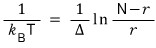
$$ \begin{aligned}\cong{}&\ln N!-\ln r!-\ln(N-r)!+\ln r^s-\ln(N-r)^s\\\cong{}&\ln\left[\frac{N!}{r!(N-r)!}\cdot\frac{r^s}{(N-r)^s}\right]\end{aligned} $$$$ \therefore\quad\ln\Omega(E-\varepsilon)\cong\ln\left[\frac{N!}{r!(N-r)!}\cdot\frac{r^s}{(N-r)^s}\right] $$$$ \begin{aligned}\Omega(E-\varepsilon)&\cong\frac{N!}{r!(N-r)!}\cdot\frac{r^s}{(N-r)^s}\\&\cong\Omega(E)\cdot\frac{r^s}{(N-r)^s}\end{aligned} $$

The temperature $T$ of the system satisfies $\frac{1}{k_BT}=\frac{1}{\Delta}\ln\frac{N-r}{r}$ —show this.

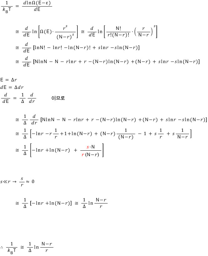
$\frac{1}{k_BT}=\frac{d\ln\Omega(E-\varepsilon)}{dE}$: here we will use the approximate expression for $\Omega(E-\varepsilon)$.

$$ \begin{aligned}\frac{1}{k_BT}&=\frac{d\ln\Omega(E-\varepsilon)}{dE}\\[1em]&\cong\frac{d}{dE}\ln\left[\Omega(E)\cdot\frac{r^s}{(N-r)^s}\right]\\&\cong\frac{d}{dE}\ln\left[\frac{N!}{r!(N-r)!}\cdot\left(\frac{r}{N-r}\right)^s\right]\\&\cong\frac{d}{dE}[\ln N!-\ln r!-\ln(N-r)!+s\ln r-s\ln(N-r)]\\&\cong\frac{d}{dE}\bigl[N\ln N-N-r\ln r+r-(N-r)\ln(N-r)\\&\qquad\qquad+(N-r)+s\ln r-s\ln(N-r)\bigr]\end{aligned} $$

Since

$$ \begin{aligned}E&=\Delta r\\dE&=\Delta\,dr\\\frac{d}{dE}&=\frac{1}{\Delta}\frac{d}{dr}\end{aligned} $$$$ \begin{aligned}\cong{}&\frac{1}{\Delta}\frac{d}{dr}\bigl[N\ln N-N-r\ln r+r-(N-r)\ln(N-r)\\&\qquad\qquad+(N-r)+s\ln r-s\ln(N-r)\bigr]\\\cong{}&\frac{1}{\Delta}\left[-\ln r-r\frac{1}{r}+1+\ln(N-r)+(N-r)\frac{1}{N-r}\right.\\&\qquad\qquad\left.-1+s\frac{1}{r}+s\frac{1}{N-r}\right]\\\cong{}&\frac{1}{\Delta}\left[-\ln r+\ln(N-r)+\frac{\textcolor{red}{s}\cdot N}{\textcolor{red}{r}(N-r)}\right]\end{aligned} $$$$ s\ll r\ \to\ \frac{s}{r}\approx0 $$$$ \begin{aligned}\cong{}&\frac{1}{\Delta}[-\ln r+\ln(N-r)]\\\cong{}&\frac{1}{\Delta}\ln\frac{N-r}{r}\end{aligned} $$$$ \therefore\quad\frac{1}{k_BT}\cong\frac{1}{\Delta}\ln\frac{N-r}{r} $$

Separate editorial clarifications

These clarifications are additions to the translation, not statements from the historical note.

1. The original normalization attempt

The normalization equation above does work. If “blah-blah” is a common coefficient $A$, then $1=A(1+e^{-\varepsilon/(k_BT)})$, so $A=1/(1+e^{-\varepsilon/(k_BT)})$. The author’s rejection is retained as part of the original working.

2. Weights, probabilities and the partition function

The ratios above use $P$ for both unnormalized weights and normalized probabilities. More clearly, use weights $w_0=1$ and $w_\varepsilon=e^{-\beta\varepsilon}$, with $\beta=1/(k_BT)$, partition function $Z=w_0+w_\varepsilon$, and probabilities $p_i=w_i/Z$. These are two nondegenerate states; $Z$ is their normalization sum, rather than a probability. The displayed mean and variance follow from these probabilities. MIT: Notes on the Canonical Ensemble.

3. Height probabilities and the atmosphere model

For a continuous height, “probability at $z$” means a probability density or a probability for a specified height interval. The count ratio is meaningful for equal-thickness bins of equal cross-sectional area; $n(z)$ can instead denote number density. The isothermal ideal-gas result $n(z)/n(0)=e^{-mgz/(k_BT)}$ assumes constant positive $T$, constant $g$, and one molecular mass $m$. Kinetic energy is still present, but integrating over velocities leaves this height dependence. Absolute normalization depends on the domain and measure. MIT: Vertical Structure of the Atmosphere.

4. The short gravitational Boltzmann factor

The short factor printed above is $e^{-z/(k_BT)}$. It is missing $mg$: for the gravitational potential energy $mgz$ used in the preceding calculation, the dimensionless Boltzmann factor is $e^{-mgz/(k_BT)}$. The longer density formula already includes this factor.

5. Constituents and the exact counting domain

The binomial count describes $N$ distinguishable constituents, each with two nondegenerate levels $0$ and $\Delta>0$; $N$ is not the number of microstates of the whole system. With integer $0\le r\le N$ excited constituents, $E=r\Delta$ and $\Omega(E)=\binom Nr$. Removing $\varepsilon=s\Delta$ requires an integer $0\le s\le r$, giving $\Omega(E-\varepsilon)=\binom N{r-s}$.

6. Stirling signs and the finite energy exchange

Use $\ln n!\simeq n\ln n-n$ when $n$ is large. The colored “+0” line is preserved literally, but its individual bracket-to-factorial substitutions do not have these Stirling signs. Their total linear discrepancy cancels because $N=r+(N-r)$; this does not validate each substitution separately. An exact anchor for the final ratio is

$$ \frac{\Omega(E-\varepsilon)}{\Omega(E)}=\prod_{j=0}^{s-1}\frac{r-j}{N-r+j+1} $$

The approximation $[r/(N-r)]^s$ needs an interior regime with both $r$ and $N-r$ large. Conditions $s\ll r$ and $s\ll N-r$ control each factor; good relative accuracy of the whole product also needs the accumulated log error, of order $s(s-1)/(2r)+s(s+1)/(2(N-r))$, to be small. For fixed $s$ this holds in the thermodynamic interior. For example, $N=100,r=99,s=1$ gives an exact ratio $99/2$, whereas the printed approximation gives $99$.

7. The energy at which temperature is evaluated

The usual Boltzmann-entropy definition is $\beta(E)=1/(k_BT(E))=(\partial\ln\Omega(E)/\partial E)_{N,\Delta}$. With a fixed removed energy $\varepsilon$, differentiating $\ln\Omega(E-\varepsilon)$ instead evaluates $\beta(E-\varepsilon)$. Within the leading Stirling approximation, the source’s positive additional term is $(1/\Delta)sN/[r(N-r)]$, consistent with the first small-$s$ shift of $\beta$. Dropping it requires both $s/r$ and $s/(N-r)$ to be small; to preserve relative accuracy or the sign of the leading inverse temperature, it must also be small compared with $|\ln((N-r)/r)|$. That comparison fails near the midpoint where the leading logarithm vanishes. Keep the source term and the subsequent omission visible.

8. The midpoint and negative temperatures

In the large-system interior, the Boltzmann-entropy approximation gives $\beta\simeq(1/\Delta)\ln((N-r)/r)$. It is positive below $r=N/2$, zero at the midpoint, and negative above it. Zero inverse temperature is the infinite-temperature limit, not $T=0$. Negative temperatures describe the population-inverted branch of a bounded two-level spectrum; they do not apply to the unbounded-energy isothermal atmosphere. At $r=0$ or $r=N$, the continuum/Stirling derivative is a limiting expression rather than an exact finite-system derivative. MIT: Statistical Mechanics I, Lecture 12.

Original source image archive

All 25 unmodified native image occurrences, retained in original order. The English and native-math reconstructions above preserve their substantive content.