Expected Speed, Expected Energy, and Statistical Analysis of Ideal Gas Speed

Alright, so let’s stop talking about distributions now. Now we’re going to look at averages. So let’s look at velocity again.

This time, let’s again put ‘one’ gas molecule into a system at temperature $T$. The probability density for this molecule’s x-component of velocity, , is

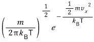
We organized this already in the velocity-distribution post. Now we’re going to measure one molecule in a system at temperature $T$!

What expectation value do we get for that measurement?

Here’s the add-it-all-up sketch:

You just add the contributions up like this! But $g(v_x)$ is a density, so a little interval contributes $v_xg(v_x)\,dv_x$, rather than the bare density-weighted value in that sketch. Since velocity is continuous, let’s use an integral.

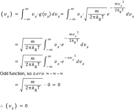
Aha, so in the gas’s rest frame, the average of the velocity component is 0. Makes sense… heh.

Ah damn! This isn’t what I was curious about! What about the average of its magnitude instead?

This thing, this one: . We integrate the earlier function, weighted by , from 0 to infinity, and multiply by 2.

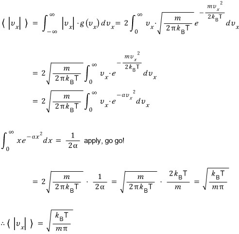
That’s how we find the mean magnitude of one velocity component. The correct result is $\langle |v_x|\rangle=\sqrt{2k_B T/(m\pi)}$.

Let’s also get the average of that component squared!

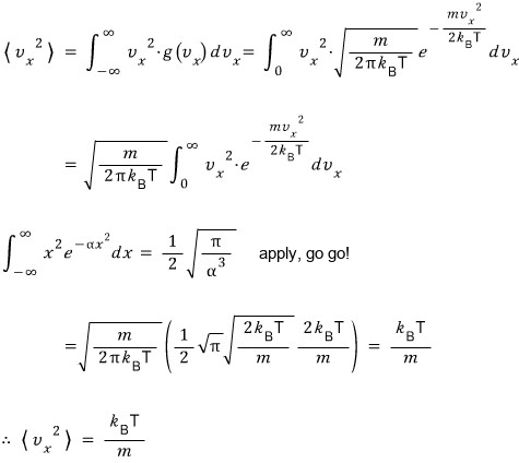
So like this, we’ve done everything for , but this was just practice ^^. It was practice for what we’re about to do.

What’s more meaningful for us is finding the expectation values for the full speed, without picking a direction.

Earlier it was , and now we’re doing it for the full, direction-independent speed, .

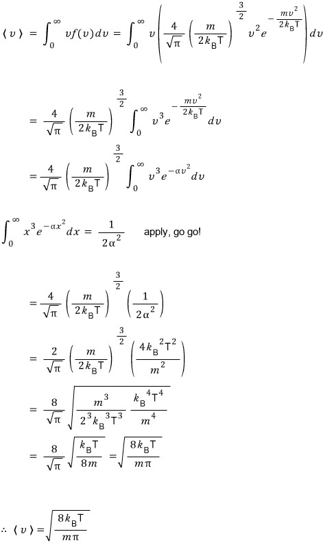
It looks somewhat complicated, but since you just need to do a little cancel-to-the-ation, it’s not hard. Let’s also find the average of . Since we have a kinda-formula-kinda-not-formula, there’s nothing to be scared of.

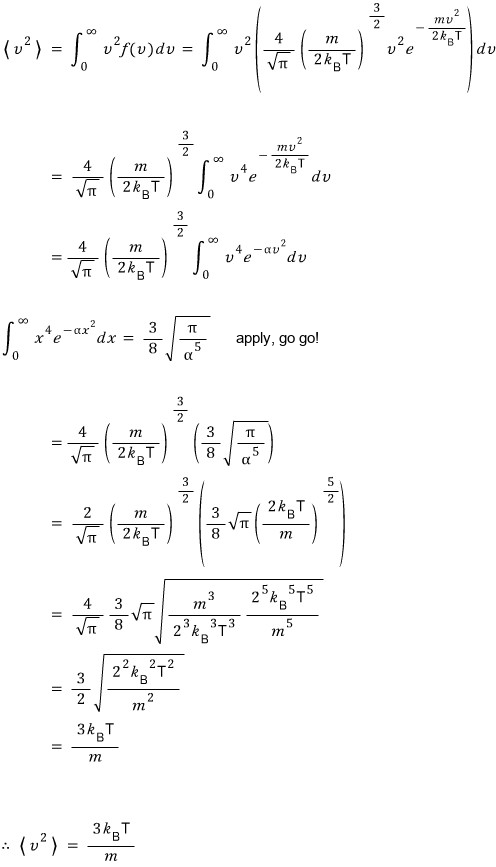
Do you remember getting 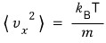?! The fact that we got 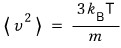means

this was the case!

And what if you take the mean of the square and “put a square root on it…”?

That’s exactly the root-mean-square (rms) value!

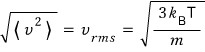
They say to pay attention to the fact that, at the same temperature, the rms speed is inversely proportional to the square root of mass!

That’s the same mass dependence we learned about in Graham’s law of effusion in chemistry class, and it’ll come up later for us ^^. Since it’s content that’ll appear then, I think that’s why they told us to pay attention.

Let’s also find the average of translational kinetic energy, .

This is a calculation we’ve already done above… heh.

I learned this in Physics 2 class!

The mean translational kinetic energy per molecule depends ONLY on temperature! That’s what we learned! Hehe.

The integrals needed in the “apply, go go!” steps above are in the earlier integral post.

Don’t forget. The assumption of an ideal gas came along, and the assumption of following the Boltzmann distribution came along.

---

Heads-up. The figures here are the original notes, slips and all. A few things to watch for:

• In the picture for $\langle |v_x| \rangle$, the last steps lose a factor $\sqrt{2}$: $2\sqrt{\frac{m}{2\pi k_B T}}\cdot\frac{1}{2\alpha} = \sqrt{\frac{2k_B T}{\pi m}}$, so $\langle |v_x| \rangle = \sqrt{2k_B T/(\pi m)}$, not $\sqrt{k_B T/(m\pi)}$.
• In the picture for $\langle v_x^2 \rangle$, the first two lines integrate from $0$; the integral runs over all $v_x$ from $-\infty$ to $\infty$, which is also the formula applied next. The result $k_B T/m$ is right.
• In the picture for $\langle v^2 \rangle$, one middle line has $2/\sqrt{\pi}$ in front; it stays $4/\sqrt{\pi}$, as the next line shows. The result $3k_B T/m$ is right.