Bose-Einstein and Fermi-Dirac Distributions
Switching gears to talk about quantum distributions — what makes bosons and fermions different, and why spin and the Pauli exclusion principle totally change the game!
This time I’m going to switch up the order a bit and talk about distributions first.
We’ve been dealing with ‘gases’ all this time, and we said gases follow the “Boltzmann Distribution”, right?!?!
But in the quantum world, that distribution is a liiiittle different.
First of all, basically, for identical particles (particles that are the same, particles that can’t be distinguished), quantum physics classifies them into two types.
Namely bosons and fermions.
How are bosons and fermions classified?!?!!?!
A boson is a particle with integer spin.
For example, a photon with spin 1, or helium made of 2 neutrons with spin 0

there’s that.
And what’s called a fermion is a particle with half-integer spin.
Things like electrons, protons, neutrons, which have spin 1/2!!!!
Then the fundamental difference that arises between having integer spin and half-integer spin
lies fundamentally in whether or not they follow the Pauli exclusion principle,
bosons do not follow the Pauli exclusion principle, and fermions do follow the Pauli exclusion principle!!!!
I’ll chat a bit about the above, and then we’ll get into the real discussion!!!
First of all, basically identical particles are… identical, so they can’t be distinguished….(obviously…T_T)
So what I mean is, http://gdpresent.blog.me/220575502936
Quantum Mechanics as I Studied It #26. 2 Particles and Exchange Force
Alright… finally. chapter 5. Up to this point we’ve totally finished up with the hydrogen atom.(it was insanely long …
blog.naver.com
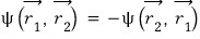
Not a situation like this,,,
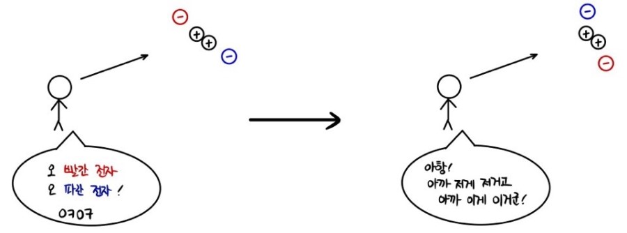
I’m saying it’s a situation like this.
That is,

this wavefunction and

these two wavefunctions just can’t be distinguished at all.
Not being able to be distinguished means that the “probability density functions”, which are the squares of the two wavefunctions, are the same!!!
That is,
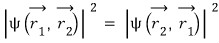
that’s what it means
therefore
we can reach this conclusion.
You can also derive the above equation with different logic.

and

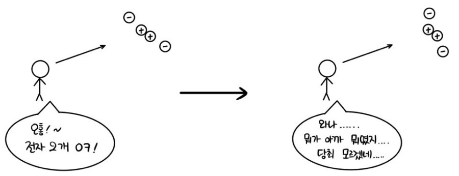
not being distinguishable means that
The probability density functions of the two wavefunctions should be equal, but
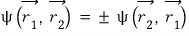
To make that happen, must the two wavefunctions absolutely be the same?!?!?!

Do they have to be exactly the same like this?
No No that’s not it, even if the two wavefunctions just differ by a ‘phase’, we can still say the probability density functions are the same
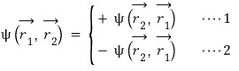
Therefore
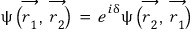
we can write an equation like this
The real numbers that the exponential term can take are 1, -1
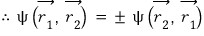
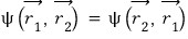
That is, for the ’exchange’ of swapping the positions of the particles, two things are possible.

Equation 1 is called symmetric, and the particles that have this characteristic are bosons
Equation 2 is called antisymmetric, and the particles that have this characteristic are fermions.
I won’t go through why bosons follow equation 1 and why fermions follow equation 2 here.
However I’ll just touch on the point that following equation 1 means not following the Pauli exclusion principle,
and following equation 2 means following the Pauli exclusion principle.
Let’s say two particles can each be in |0> or |1>.
If the two particles are distinguishable?!?!~~~(distinguishable)
|0>|0>, |0>|1>, |1>|0>, |1>|1> all 4 of these possible situations will be ‘different’ states.
But, if the two particles are indistinguishable, the possible states are not those 4, but
|0>|0>, |0>|1>,,|1>|1> these 3, we’d have to say
But if those 3 follow the symmetric
that is
if they have to follow this,
|0>|0> = |0>|0>
|1>|1>
these hold automatically, whereas
|0>|1> will be a state where the probabilities are fused together.
|1>|0>
Including the normalization constant that requires 1 squared to be 1
|1>|0>
Alright alright alright alright alright so the 3
state functions of a two-level system that satisfy the symmetric wavefunction are
|0>|0>
|1>|1>
|1>|0>
these 3.
Then, the antisymmetric wavefunction
if it has to follow this
|0>|0> is impossible
|0>|0> = -|0>|0>
for this equation to hold
um
the value of A that makes A = -A hold is only what???only 0, right?
Therefore |0>|0> = 0 and |0>|0> is not possible.
It doesn’t exist. That’s what it means.
Likewise |1>|1> also doesn’t exist as an antisymmetric wavefunction.
That is, the Pauli exclusion principle that “the same quantum state cannot coexist in one state” was this,
and in a two-level system the only quantum state that antisymmetric allows is |0>|1>.
But, |0>|1> and -|1>|0> will look the same,
so the two states will look like one “probability” (one wavefunction).
(probability of |0>|1>) + (probability of -|1>|0>)
And since the square of the wavefunction has to be 1 (normalization condition)
the state allowed by the antisymmetric wavefunction is
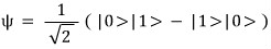
just this one…hehe
Then the basic concept talk ends here.
Now let’s go to statistical physics.
Let’s go to the main topic, the Bose-Einstein distribution and the Fermi-Dirac distribution.
This kind of difference has a huge impact on statistics.
How does it have a different impact?!?!
Let’s look at the difference by calculating the partition function.
To look at it in the most general way, we’re going to consider it in the Grand canonical ensemble.
The definition of the partition function in the grand canonical ensemble was
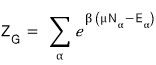
this.
It’s important that α means energy state

you can think of it as the number of particles in the α-state

you can think of this as the energy in the α-state.
<You shouldn’t get confused about the meaning of α. It doesn’t mean the energy level, but
rather the energy kind?! that it can have, like a rotational energy term, translational kinetic energy term, quantum energy term and so on~~!!!>
Alright now, first let’s say only 1 state is possible.
We have to count all possible cases that can occur in that single state
In this one possible state, when there’s 1 particle, 2 particles, 3 particles,…. let’s count every case.
When the count is 1, N is N=1, and at that point the energy is E
When the count is 2, N=2, and since there are 2, the energy is 2E
When there are k, N=k, and since there are k, the energy is kE
That is,
And the expected value < n > for the number of particles is
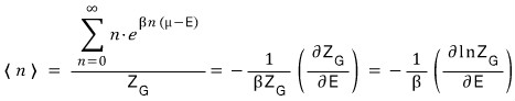
it ends up organized like this?!?!?!
Alright, but if the particle is a fermion, n can only be 0 or 1
we said more than 2 can’t be in the same quantum state
Therefore when the particle is a fermion
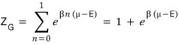
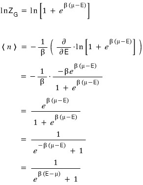
When the particle is a fermion, the partition function has been derived!!!!!
Now let’s find the expected value for the number of particles
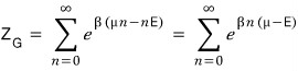
On the other hand, when the particle is a boson
n is indiscriminately allowed to be anything.
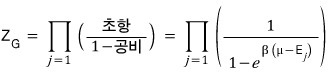
Therefore the partition function is
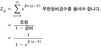
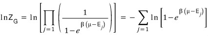
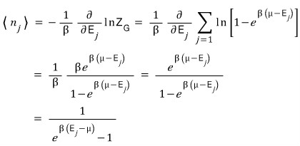
So now to find the expected value for the particle,
I’ll take the log of that partition function, ~~~ take the partial derivative with respect to E ~~~~ and multiply by 1/(-β).
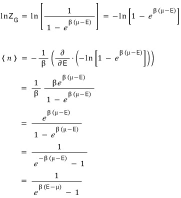
Eek!!! The shape came out almost~~ identical to the Bose-Einstein & Fermi-Dirac distributions we knew beforehand!??!?!!!
Then this time let’s derive it a bit more generally!!~
We’re going to throw away the assumption that only 1 state is possible and derive it again.
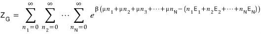
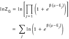
The definition of the partition function is

this
we said α means state.
First, the whole system has a total of N particles,
let’s think of it this way
There are state 1, state 2, state 3, . . . ., state N,
in state 1 there are

particles
in state 2 there are

particles
in state 3 there are

particles
rowwwww after row, and since we said the whole system has N particles,

this is correct.
Alright and
if you enter state 1, you get an energy of

and there are

particles there, so the energy from state 1 is

if you enter state 2, you get an energy of

and there are

particles there, so the energy from state 2 is

if you enter state 3, you get an energy of

and there are

particles there, so the energy from state 3 is

rowwwwwww after row
Thinking up to here, the exponent term of the partition function’s exponential
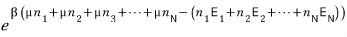
will be this kind of shape.
But here’s the thing.
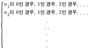
There are way too many cases to consider
Anyway….. since it’s an unavoidable fact that we have to count them all, the partition function has to be written like this.
While not a difficult equation, it’s obnoxiously long and looks like it’ll totally break your mental
when it’s nothing at all -_-
After tidying up the equation to look nice,
I’ll now shut my mouth and just drag the equations down.
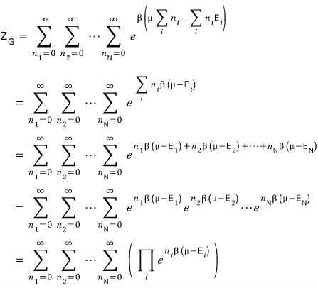
Up to here no problems, right….?T_T T_T T_T
Then I’ll keep going with the shenanigans.
I’m not that smart so I’ll go as detailed as possible T_T T_T T_T
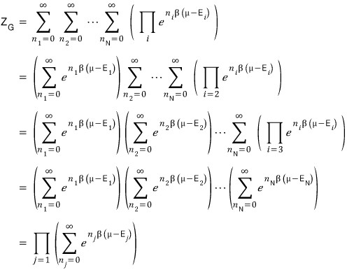
Done!!!!!! If we tidy it up like this, we’re all done.
Now all that’s left is to compute the thing that looks complicated above for the fermion case and the boson case.
But, it’s not complicated at all!!!~~
In the case where the particle is a fermion, by the Pauli exclusion principle

is only allowed to be 0 or 1.
Therefore
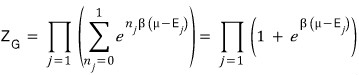
Then
This time we’re not partial differentiating with respect to E, but partial differentiating with respect to E_j.
A relation for “the number of particles at each energy level” will come out!!!lol lol lol
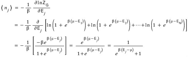
Interpreting the meaning, for a particle and system with temperature T and chemical potential μ
in the j-th state, on average there are this many fermions!!!! we could say.
Let’s go with bosons too.
Since bosons have no limit on the number of particles in each state
the partition function has to go through the following operation.
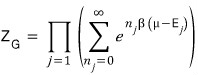
So we have to compute an infinite geometric series again.
That is,
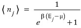
So the expected value for the number of particles at each energy level is
Interpreting the meaning of this one again, for a particle and system with temperature T and chemical potential μ
in the j-th state, on average there are this many bosons!!!! we could say~~~
Woohoo~~~
Originally written in Korean on my Naver blog (2016-06). Translated to English for gdpark.blog.