Brownian Motion and the Langevin Equation

Around middle school??? you probably encountered Brownian motion.

At school, you dropped a drop of ink plop-plop into water, right????

What happened to the liquid??? It spread ou~~~t~~~ all over the place.

It just spreads out, and these things spread randomly, right????

So, if you drop ink again under the same conditions, does it show the exa~~ctly same behavior as before??

Probably not. It’s going to spread out in a different shape than before, isn’t it?????

So it’s fine to say it spreads randomly.

OKOK, now let’s study this stuff roughly.

For the details, go to graduate school^^

Then let’s get started!!!!

As I said above, the first person to study this random behavior was the Scottish botanist “Robert Brown.”

The year of the research was 1827.

Robert Brown was the first to study it, but he wasn’t the first to discover it.

Anyway, Brown was doing an experiment floating pollen in water and observing it during some research unrelated to random behavior,

and he discovered that the pollen grains moved randomly.

But the scholar who had discovered this earlier had called it “a living, moving creature (microbe) inside the liquid,”

i.e., a kind of ’life force,’ it’s said.

But Brown thought “Ah… is this the pollen’s life force????” and then

he tried putting in glass, metal, stone, etc. ground as small as pollen, and—

“What the!!!!!!!!!!!!!!!!!! It’s exactly the same as pollen!!!!!!!!!!!!!!!!”

so he discovered this and studied this kind of behavior, it’s said.

That is, what he revealed was something like “it’s not a life force.”

Makes sense. In the early 1800s there wasn’t even the concept of ‘atoms’ yet,

and it was an age when protons, neutrons, and electrons couldn’t even be dreamed of.

And then afterwards, with the development of thermodynamics, people pointed to “convection” as the cause of Brownian motion.

Since Brownian motion in hot water is more active than in cold water, they pointed to convection as the cause,

but that still couldn’t be a perfect explanation.

And in further follow-up research, the cause of Brownian motion was revealed to be “collisions by liquid molecules,” it’s said.

This could be said to be because the discovery of particles and the development of statistical physics starting with Boltzmann ran in parallel.

And then in 1905, the miracle year came.

1905 is called the miracle year because Einstein announced 4 papers to the world at once that would astonish the world,

and among those 4 papers, one was about Brownian motion, it’s said. (The other 3 would be special relativity, the photoelectric effect, and mass-energy equivalence)

And in 1906, Poland’s Marian Paul Smoluchowski, with an approach totally different from Einstein’s approach,

precisely derived Einstein’s formula, and this theory was proven experimentally by French physical chemist Perrin in 1908,

stamping it with the ’truth’ seal. (The Nobel Prize in Physics went to Perrin….heh)

Alright, then we’re going to start Brownian motion.

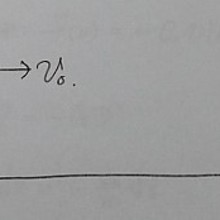
Let’s get a feel with just this much of a picture and go.

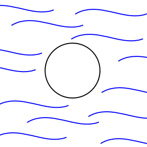
Why doesn’t the big disk floating on top of the water

move around every which way like the pollen grains?!?!?!?!?!!!

It’s because, since the object is large, the “random forces” acting from various directions will be felt as net zero.

That is, they’ll be felt as a uniform force hahahaha

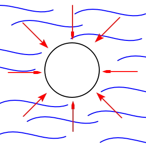
Then why does the pollen?!!?!???Why do the small ones!!!!!!!!!!!!!!

Fundamentally, even if it’s a net-zero force, to particles that are too small it becomes not balanced.

So it moves around every which way, but in any case, the force that makes it move around randomly like that

is fundamentally a force whose net is zero!!!

Get a feel for this and let’s go.

Alright, now let’s go in earnest.

First, I’ll write the equation of motion for a single particle.

The equation of motion for a particle of mass m inside a fluid is

I’m going to write this,

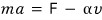
I wrote it including the damping resistance term like this.

There are many kinds of damping — velocity-dependent, velocity-squared-dependent, velocity-cubed-dependent… etc.,

but if the object is small, the velocity-dependent term is most dominant, I learned in general mechanics class. http://gdpresent.blog.me/220394492888

What I studied in general mechanics #2. Newtonian mechanics, work-energy theorem, conservative forces

Hi Newton ~!!! lollollollollollollollolfucking Bye ! ~ lollollollollollollollollollollollollolAt first something …

blog.naver.com

The force here is exactly the ‘random force’. That is, it’s a force for which < F > = 0.

It’s probably good to keep in mind the difference that it’s not the time average that is zero, but the ensemble average.

Now the goal is to find the solution x(t) of that equation.

So I’m going to rewrite it like this.

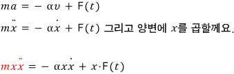
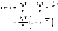
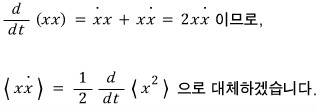
Having written up to here, I’m going to express the red guy on the left side ‘differently’ through the following equation.

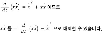
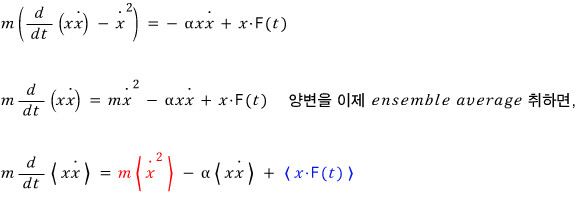
The red one, by the equipartition theorem,

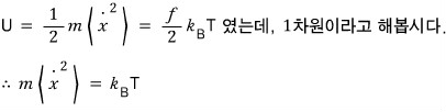
As for the blue one, since F(t) is a random force, it has no~ connection whatsoever with the position x, so separation is possible and

<xF(t)> = <F(t)>

writing it like this is fine, and because it’s a random force < F(t) > = 0, so the blue term is zero.

Therefore the above equation

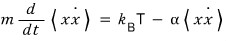
can be organized like this, and now putting it into a form suitable for solving the ODE,

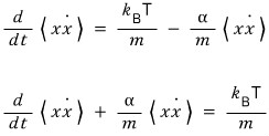
Oho?!?!? This is a first-order ODE of the form y’ + py = Q.

Setting <xx_dot> = y, I’ll solve the ODE. http://gdpresent.blog.me/220341671707

Differential equations special posting.

If you’re a college STEM undergraduate, you encounter “(linear) differential equations” a damn lot. I thought I’d do a posting about this…

blog.naver.com

I’ll follow this. If you’re curious about the principles, go look over there and come back.

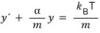
<Actually, prime denotes differentiation with respect to space, and it’s customary to put a dot for differentiation with respect to time, so the above expression is in some sense wrong. But,,, just understand it hahahaha>

First let me find the homogeneous solution.

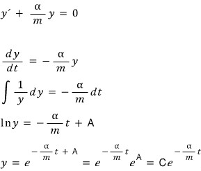
Got the homogeneous solution!!!!!

Then let’s go back to the original ODE.

Here to both sides

I’ll multiply this a bit.

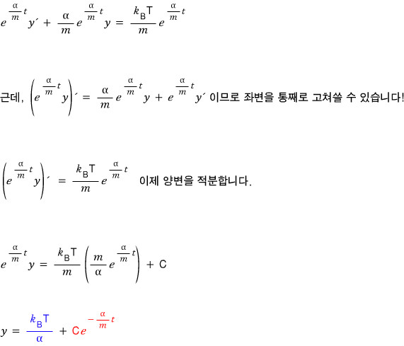
Ohhh, the red guy must be the homogeneous solution we saw above,

and the blue one must be the special solution!!!!!

Anyway, y, i.e.

we found the General Solution.

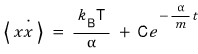
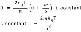
I’ll now determine that constant C.

I’m going to take t=0 initial condition x=0 to determine the integration constant C.

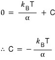
An integration constant determined in two lines lollollollollollollollollollollollollollollol

So

Now let’s go for the final goal, finding x(t)!!!!!!

Likewise, let’s determine the constant by saying x=0 when t=0.

That is,

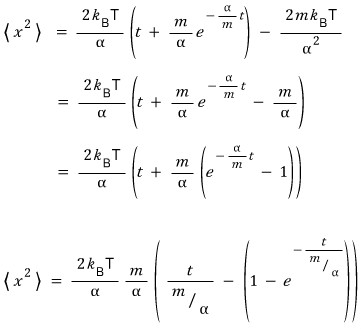
The reason I wrote it so weirdly like that at the very end is exactly

it means it’s close to 0!!! So then the front term can be ignored, so I’ll toss it out a bit?!?!?!?!

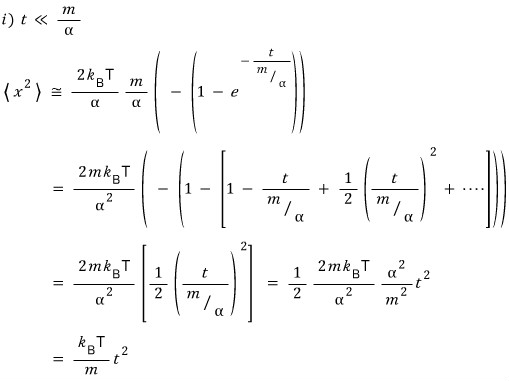
Our interest is NOT in the transient ‘moment right after starting’

time….!!!

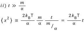
When entering the stagnation stage,

let’s focus on the fact that it’s approximated linearly in time like this.

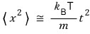
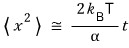
if we let this,

we can say this………uhuhuhuhhuhuhuhuhuhuhuhuhuhuhuhuh

The meaning of D!!!!!!!!!!!!!! I’ll reveal it properly in the next posting!!!!!!!!!!

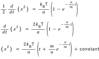
Anyway, we’ve learned that the average of the square of position x grows in a linear relationship with time t,

the ‘variance’ grows,

i.e., “it spreads”

no no “it appears to spread”

that that’s proportional to time and inversely proportional to the damping constant!!!!!!!!

And also that it doesn’t depend on mass!!!!!!!!

Well, we can draw conclusions like this much, and

now now now now now now now now now now

the meaning of this solution we just mindlessly solved the ODE and found — I’ll reveal it properly in the next posting

Keep reading!@@@@@@@@@@@@@@@@@@@@@@@@@@@@@@@@@@@@@@

Originally written in Korean on my Naver blog (2016-07). Translated to English for gdpark.blog.