Money and Banking at a Glance: Series Overview [Money & Banking I Studied #13]

At a glance! (Don’t look with both eyes, okay? >0<)

These are my 2015 study sheets for the money-and-banking series. They are a map of the textbook models, not a description of today’s policy settings. Keep the drawings beside the explanations below: the point is to see how a central-bank decision eventually reaches spending and prices.

First separate the tool from the goal

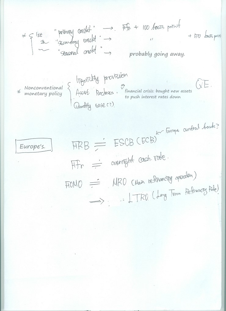
Handwritten notes on discount lending (primary, secondary and seasonal credit), nonconventional monetary policy and the ECB’s counterparts of the Fed’s tools

Discount lending, asset purchases, and refinancing operations are tools. Price stability and employment are goals. They sit at different ends of the chain; announcing a tool doesn’t tell us its final economic effect. Some labels and guesses on this old sheet are historical, too. QE means quantitative easing, and LTRO means longer-term refinancing operations.

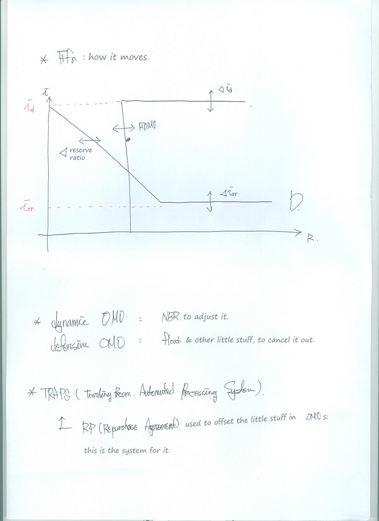
Handwritten notes on the market for reserves and the federal funds rate, dynamic and defensive open market operations, and TRAPS

The reserve-market picture asks how changing reserve supply or demand changes the overnight rate. Read it as the older textbook framework. For the current US implementation framework, see the New York Fed’s explanation: with ample reserves, administered rates do most of the work of steering the federal funds rate. Sliding a vertical reserve-supply line is not a complete account of that framework.

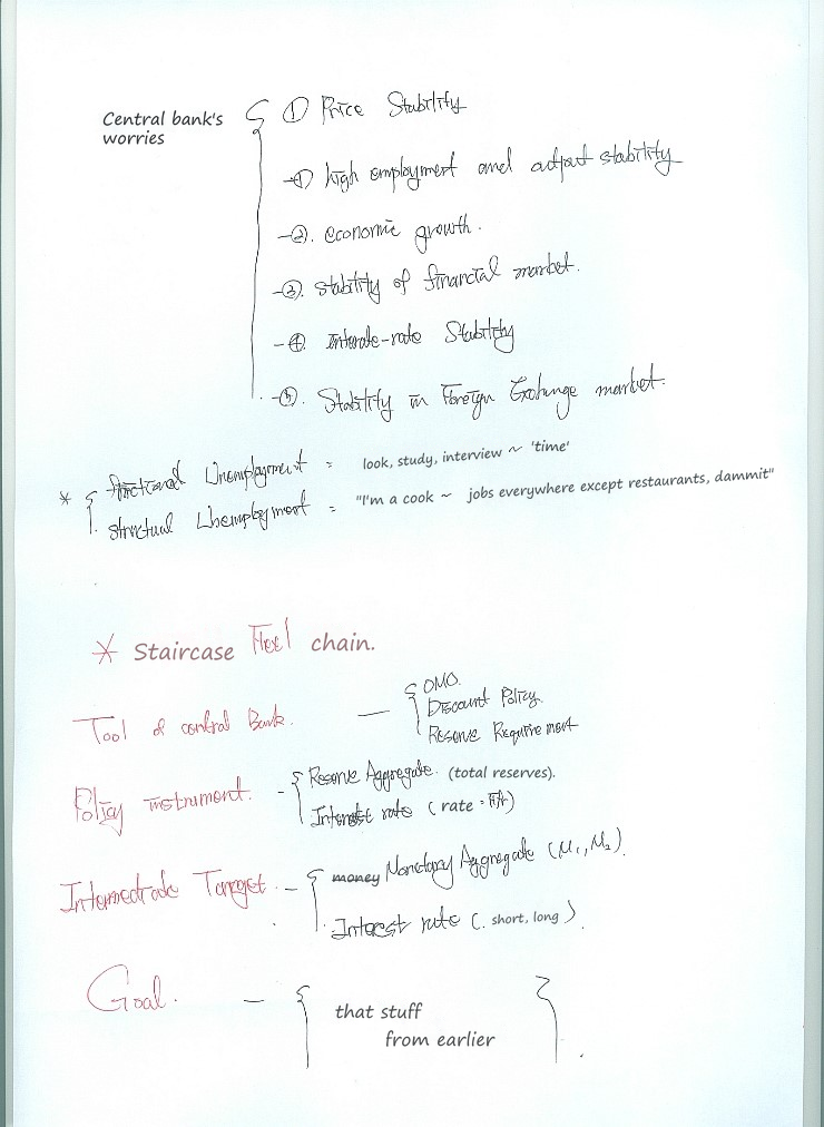
Handwritten notes on the goals of monetary policy, frictional and structural unemployment, and the chain from policy tools to goals

Here is the whole staircase: tool → operating instrument → intermediate target → goal. A central bank can change an instrument directly, while output, employment, and inflation respond through households, banks, and firms. That gap is why the transmission mechanism matters.

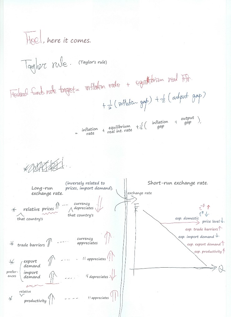
Handwritten notes on the Taylor rule and the factors that move the long-run and short-run exchange rate

The Taylor rule is a way to organize a policy-rate response to inflation and the output gap. It is a model rule, not a promise that every central bank follows these coefficients. The exchange-rate sketch beside it asks a different question: what changes the relative attractiveness of holding the two currencies?

A central-bank balance sheet is not the whole money supply

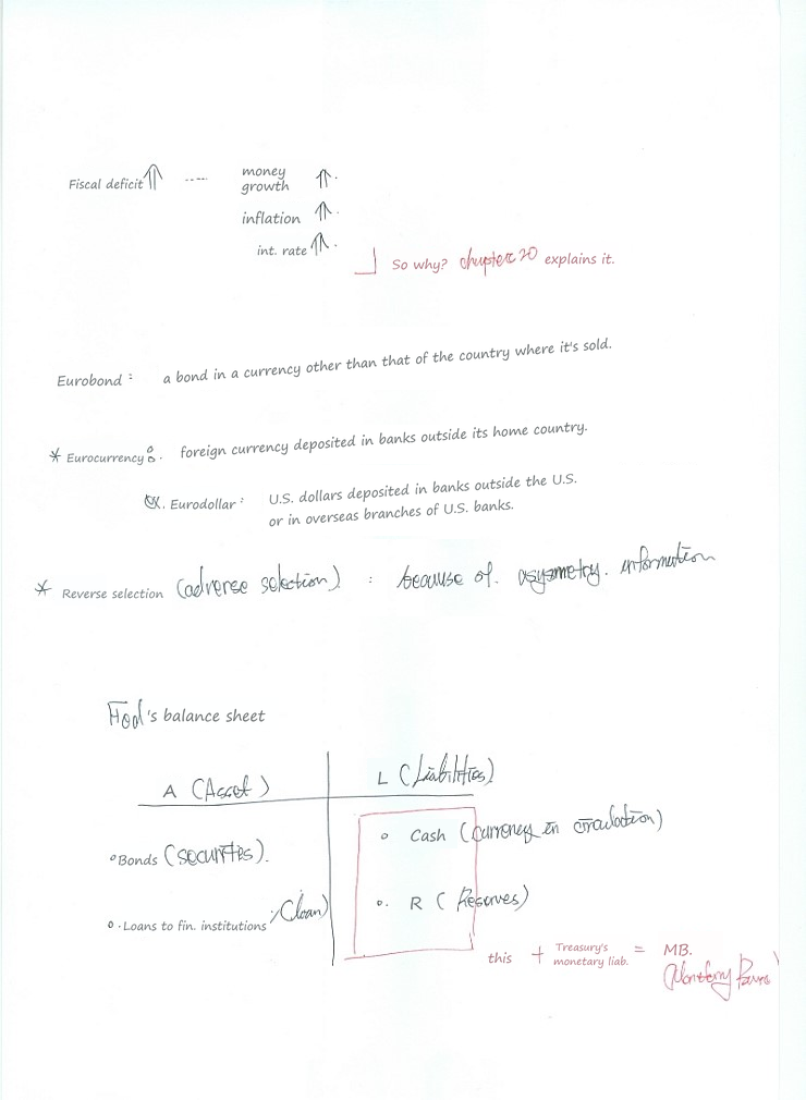
Handwritten notes on deficits and money growth, Eurobonds and Eurocurrencies, adverse selection, and the Fed’s balance sheet

On the central bank’s balance sheet, securities and loans are assets; currency and bank reserves are liabilities. Notice the distinction already: a reserve balance held by a bank isn’t a household’s bank deposit. Don’t silently swap one for the other when following an arrow.

The deficit arrow at the top is conditional. Selling government bonds to the public is not the same transaction as financing a deficit through money creation. We come back to that distinction below.

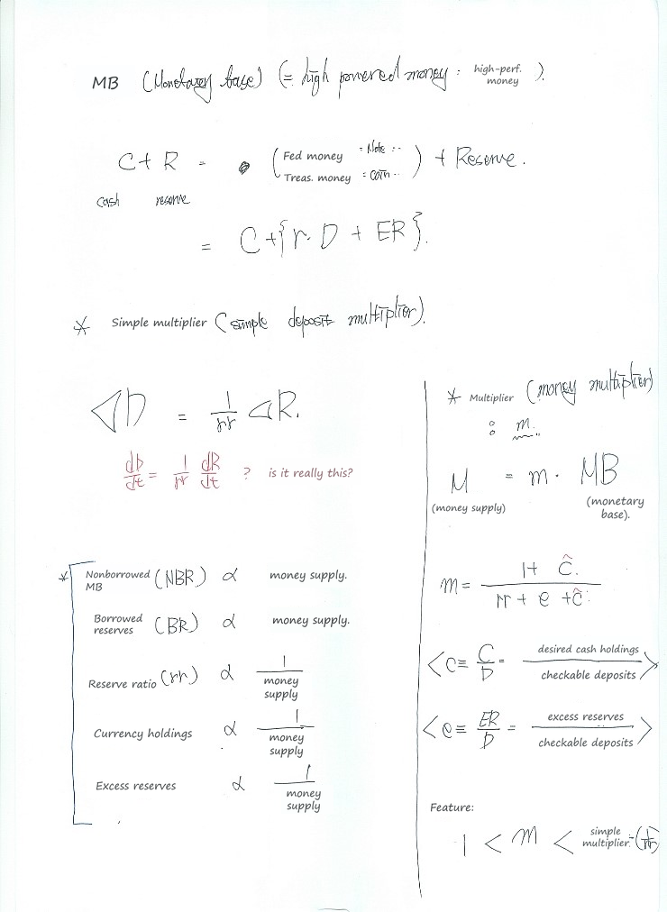
Handwritten notes on the monetary base, the simple deposit multiplier, the money multiplier and the determinants of the money supply

Write currency as $C$, deposits as $D$, and reserves as $R$. In this simplified model, $MB=C+R$ but the money measure is $M=C+D$. Set $c=C/D$, $e=ER/D$, and the required-reserve ratio to $rr$; then $R=(rr+e)D$. Dividing the two identities gives

$$m=\frac{M}{MB}=\frac{1+c}{rr+e+c}.$$

That’s where the multiplier comes from. It is not automatically greater than one: that extra claim needs $rr+e<1$. The even simpler deposit multiplier $1/rr$ also leaves out currency withdrawals and excess reserves.

Keep those assumptions attached to the equation. Actual lending is not a mechanical instruction to multiply a fixed pot of reserves; the Bank of England’s money-creation article explains how lending creates deposits and how policy constrains the process.

Exchange-rate policy has a balance-sheet side

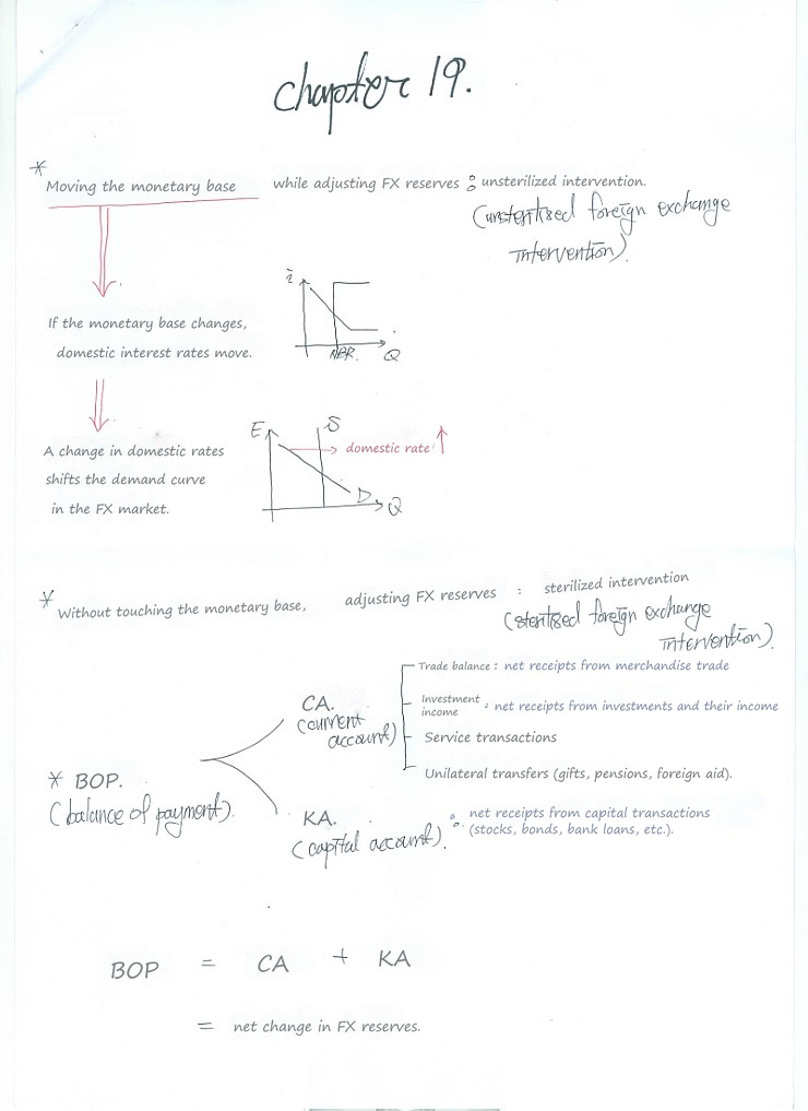
Handwritten notes on unsterilized and sterilized foreign exchange intervention and the balance of payments

Ask whether an intervention changes the monetary base. An unsterilized foreign-exchange purchase or sale lets that monetary effect remain; a sterilized intervention offsets it through a domestic operation. The balance-of-payments sketch uses an older “capital account” label for flows that modern statistics largely classify in the financial account. The full set of balance-of-payments entries balances; it isn’t just a country’s trade balance.

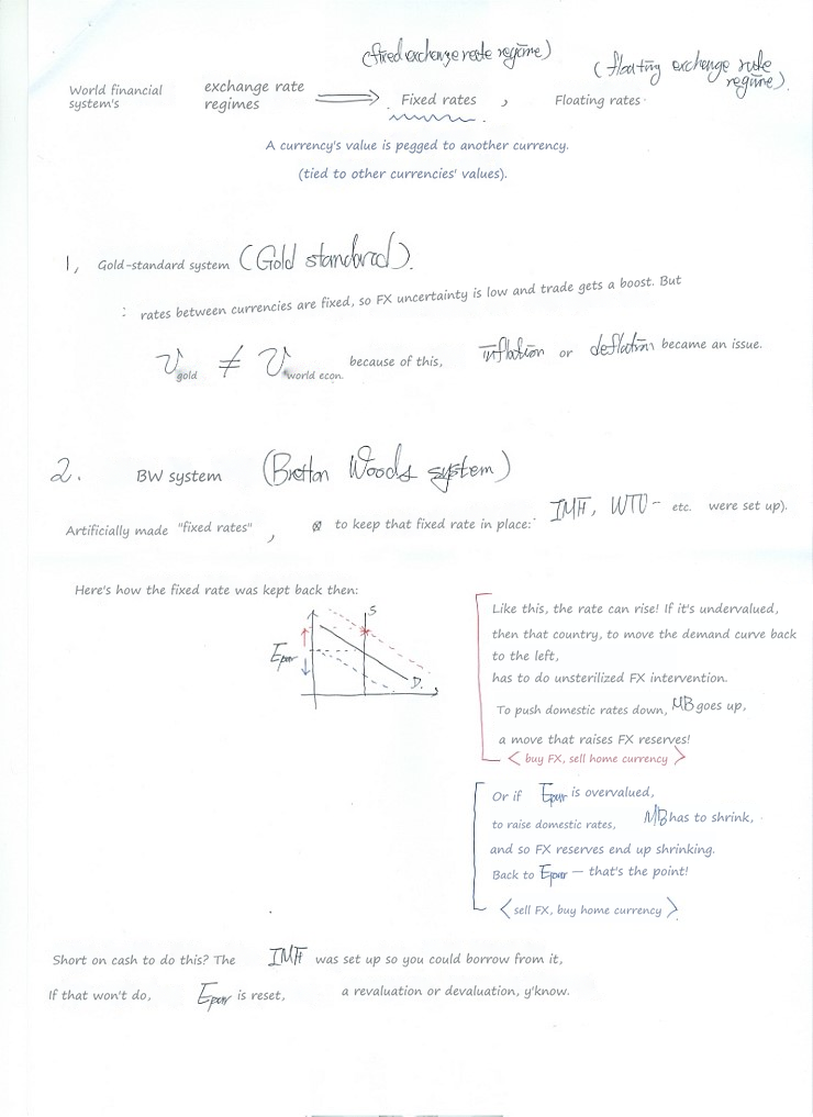
Handwritten notes on exchange-rate regimes, the gold standard and how fixed rates were kept under Bretton Woods

A fixed exchange rate requires transactions that defend the peg, rather than a declaration that the price will stay fixed. The historical examples here connect that defense to foreign reserves and the monetary base. One name needs fixing: Bretton Woods established the IMF and World Bank, not the WTO.

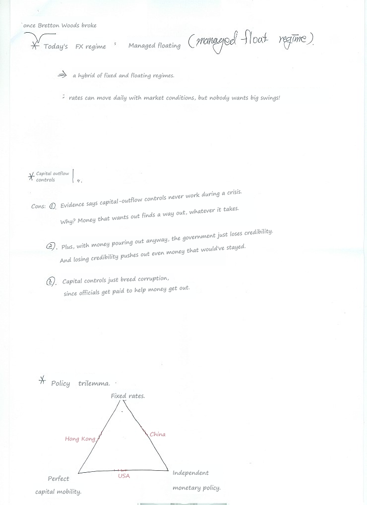
Handwritten notes on the managed float, capital controls and the policy trilemma

The trilemma is the useful organizing idea: a fixed exchange rate, free capital movement, and independent monetary policy cannot all be maintained together in the idealized framework. The country labels are examples from the old notes. Likewise, the list of problems with outflow controls is a list of possible drawbacks, not proof that controls never work.

What does the quantity equation actually tell us?

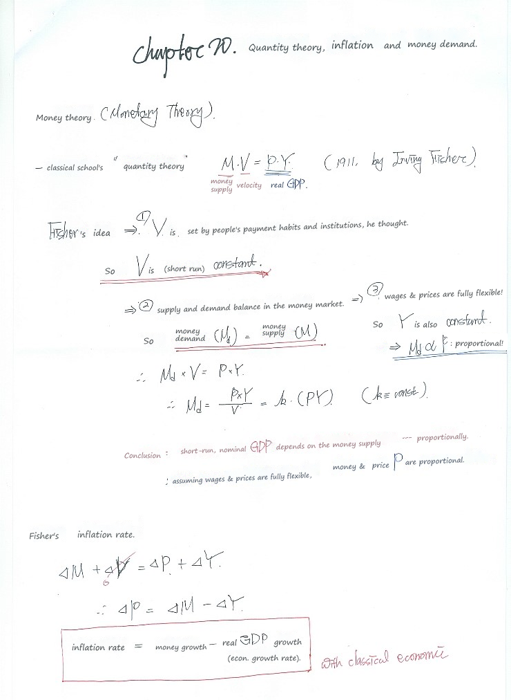
Handwritten notes on the quantity theory of money and Fisher’s inflation equation

Start with $MV=PY$: money times velocity equals nominal expenditure. The extra assumptions are what turn this accounting relationship into an inflation story. In growth-rate form, approximately,

$$\pi\approx g_M+g_V-g_Y.$$

Here $g_M$, $g_V$, and $g_Y$ are growth rates of money, velocity, and real output. Only after setting velocity growth to zero do we get the compact “money growth minus output growth” result on the sheet.

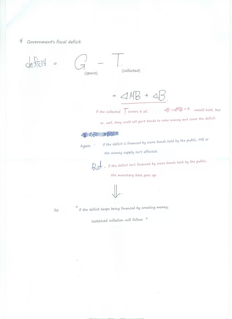
Handwritten notes on the government budget constraint and how deficits financed by creating money lead to inflation

Now revisit the deficit. The financing method matters, and so do velocity and real output. A statement about sustained monetary financing under the quantity-theory assumptions doesn’t establish that every fiscal deficit causes the same inflation outcome.

Why hold money instead of another asset?

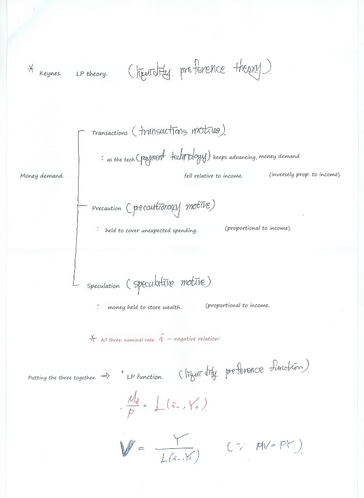
Handwritten notes on Keynes’s liquidity preference theory and the three motives for holding money

Transactions, precautions, and speculation are three ways of organizing that question. More income means more transactions to finance; it does not make transactions demand inversely proportional to income, as one line of my sheet says. Better payment technology can reduce the money needed at a given income.

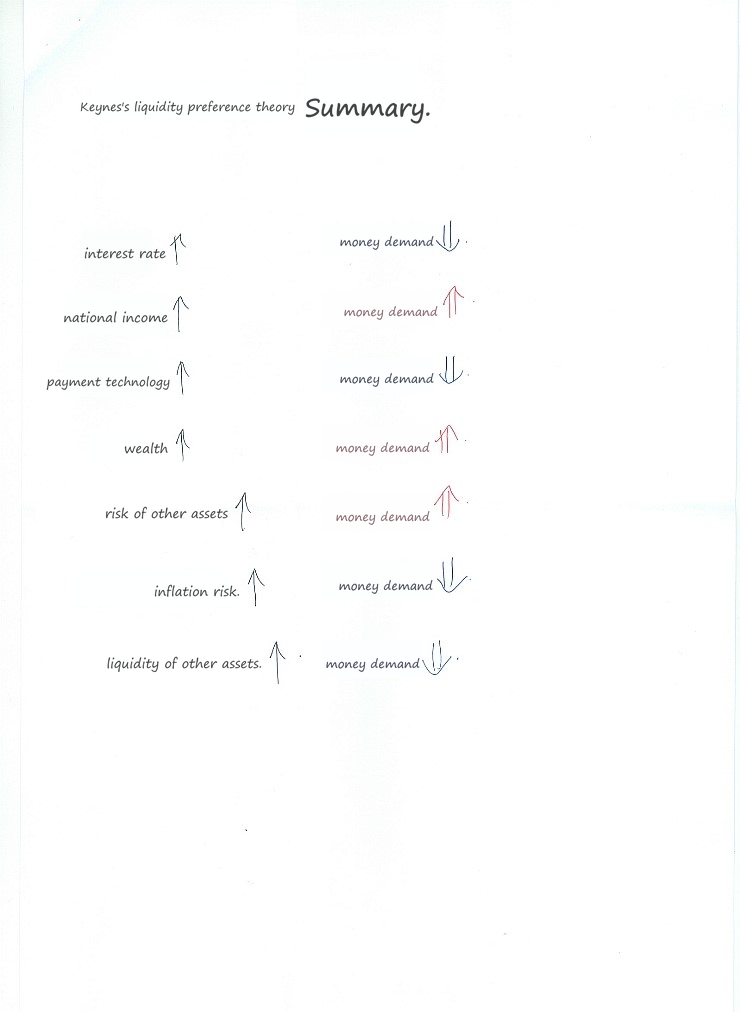
Handwritten summary table of the factors that raise or lower money demand

Read these arrows while holding the other factors fixed. A higher nominal interest rate raises the opportunity cost of holding money, whereas higher income raises money demand in this model. Mixing those two experiments together is an easy way to think the arrows contradict each other.

Connect spending to the interest-rate response

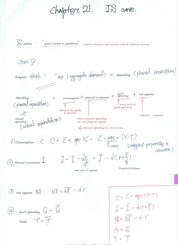
Handwritten notes on the IS curve and the components of planned expenditure

The spending pieces are consumption, planned investment, government spending, and net exports. In this setup, a higher real rate reduces interest-sensitive investment and net exports. The goods-market question is which output makes planned spending equal production.

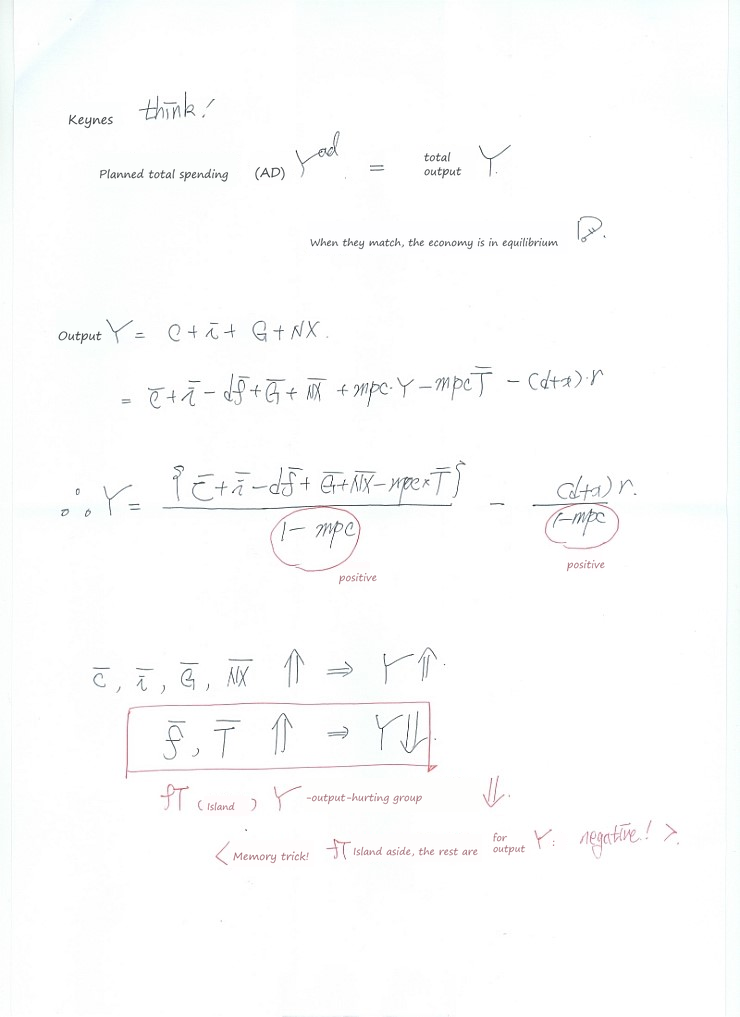
Handwritten notes on equilibrium output and the IS curve equation

With $0\lt mpc<1$, gathering the income terms on the left leaves the positive denominator $1-mpc$. That’s why higher autonomous consumption, investment, government spending, or net exports raises equilibrium output here. Higher taxes and the financial-friction term lower it. Read the signs in the equation rather than trusting the little memory note at the bottom!

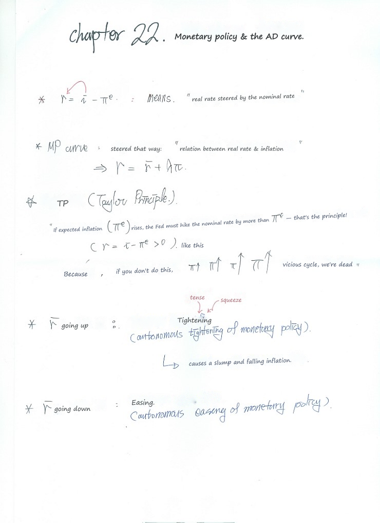
Handwritten notes on the MP curve, the Taylor principle, and autonomous tightening and easing of monetary policy

The MP curve tells us how the real rate responds to inflation: $r=\bar r+\lambda\pi$ in this version. The Taylor-principle intuition is that a sufficiently strong rise in the nominal rate makes the real rate rise when inflation rises. It is the change in the real rate that must be positive; the level needn’t always be positive.

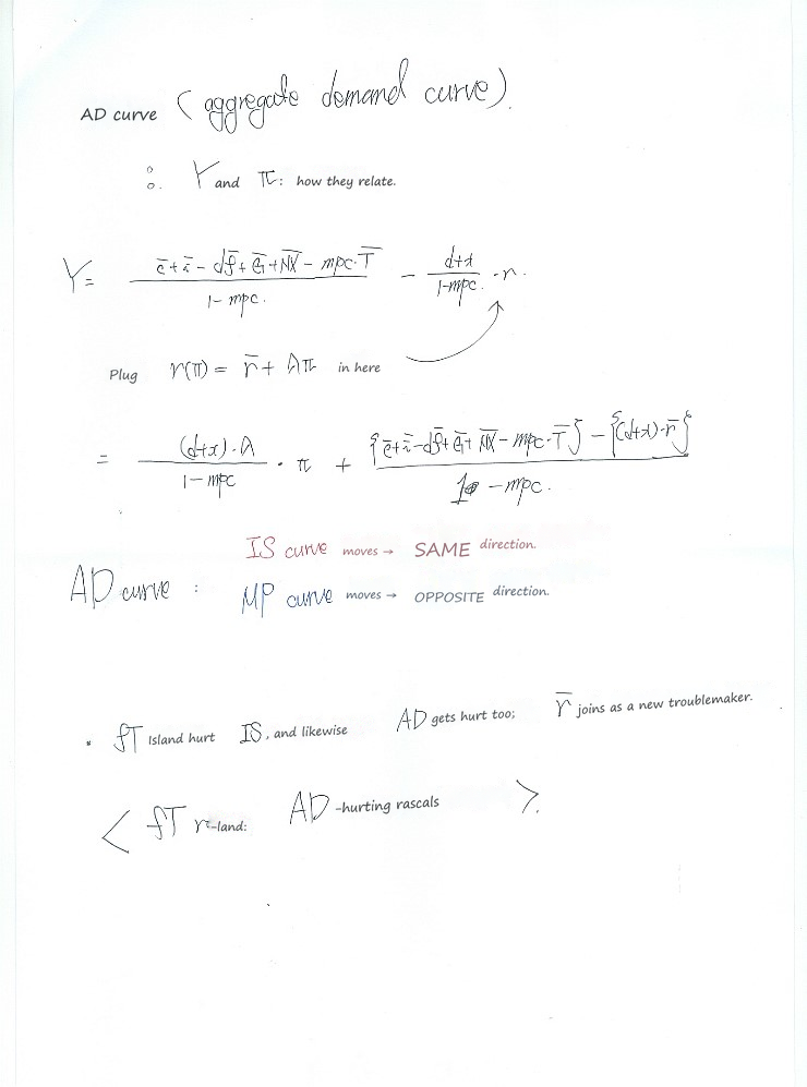
Handwritten notes deriving the AD curve from the IS curve and the MP curve

Put that policy response into the downward-sloping IS relationship. The coefficient of inflation becomes

$$-\frac{(d+x)\lambda}{1-mpc},$$

which is negative for the stated positive parameters. That missing minus sign in the drawing matters: higher inflation triggers a higher real rate, which reduces planned spending. This is the downward-sloping AD curve in the model, not a direct claim that inflation mechanically reduces every category of spending.

Demand shocks and supply shocks ask different policy questions

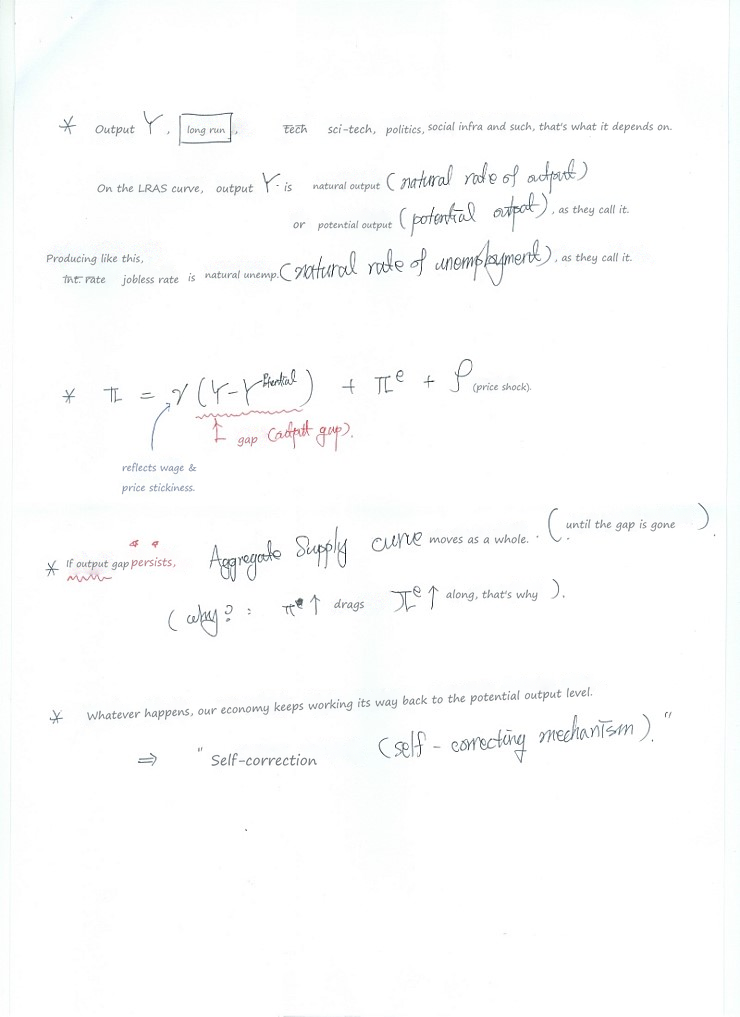
Handwritten notes on potential output, the natural rate of unemployment, the AS curve and the self-correcting mechanism

The supply side adds potential output, expected inflation, and a supply shock. The “self-correcting” path is the adjustment assumed in this particular AS–AD model. It isn’t a guarantee that a real economy returns quickly or painlessly after every disruption.

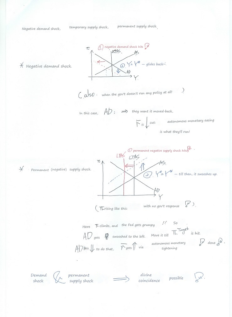
Handwritten graphs and notes on a negative demand shock and a permanent negative supply shock, with the policy responses

A negative demand shock moves spending away from potential output. A permanent negative supply shock changes the potential-output benchmark itself. Returning to the old output level is therefore not the same objective as stabilizing around the new potential level. Don’t read the “divine coincidence” shorthand as a promise of costless adjustment.

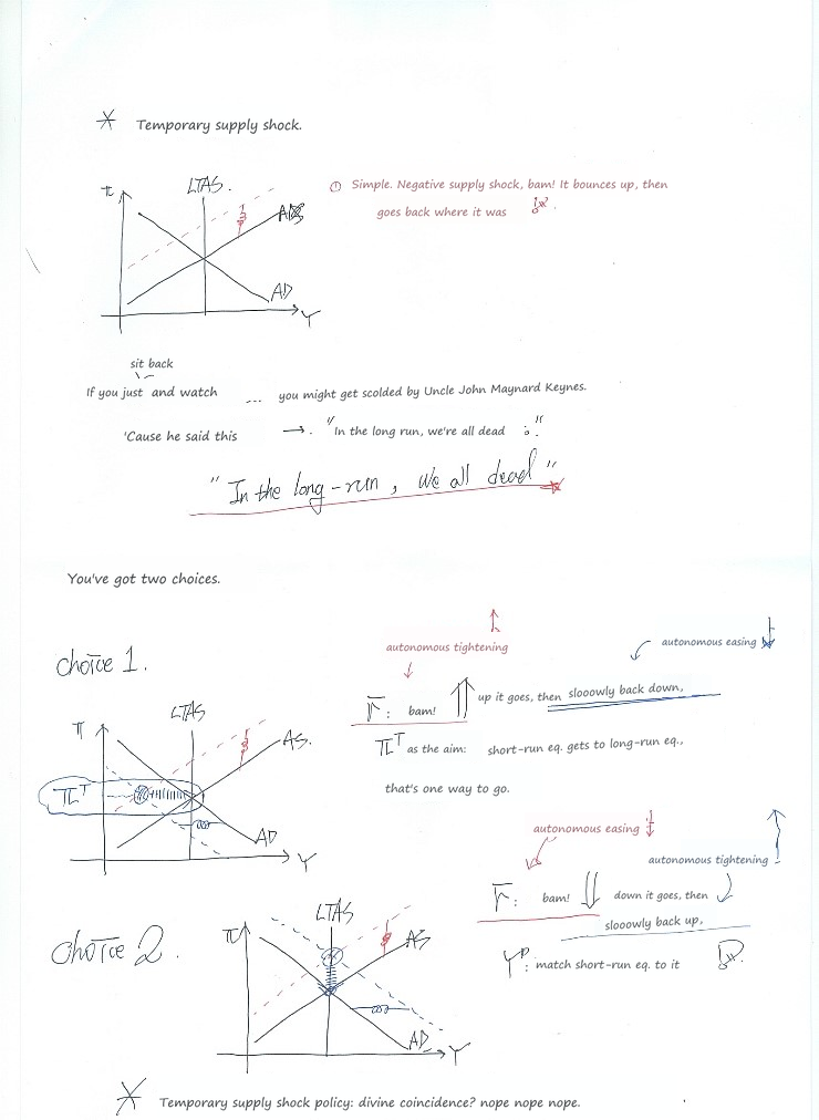
Handwritten graphs and notes on a temporary supply shock, Keynes’s long-run quip and the two policy choices

For the temporary supply shock, the drawings contrast leaning against inflation with leaning against the output loss. Follow the short-run path in each diagram, rather than looking only at its eventual endpoint. The trade-off along that path is the point of the example.

Follow one transmission channel all the way through

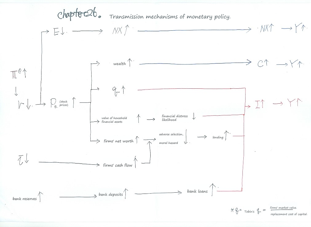
Handwritten diagram of the transmission mechanisms of monetary policy

This last sheet joins the pieces. Lower rates can affect exchange rates, asset prices, cash flow, collateral, and lending conditions; those can affect consumption, investment, and net exports. The arrows are proposed channels with assumptions, not a claim that each channel always has the same strength or timing.

Try tracing just one route aloud: lower financing costs → more investment that is worthwhile at the margin → higher planned expenditure. Then ask what could interrupt the chain, such as weak loan demand or a damaged bank balance sheet. That question is more useful than memorizing twenty arrows in one go.

For the longer explanations, return to the money-and-banking series. These sheets work best as a map after reading those notes, rather than as a substitute for every derivation.

Heads-up. The figures here are the original notes, slips and all. A few things to watch for:

In Keynes’s liquidity preference theory, transactions demand for money rises with income (it is proportional to income, not inversely proportional); what better payment technology does is lower money demand at a given income, as the summary sheet after it shows.
In the IS-curve memory note, it is $\bar{f}$ and $\bar{T}$ that lower $Y$; the other autonomous terms, $\bar{C}$, $\bar{I}$, $\bar{G}$ and $\overline{NX}$, raise it, as the arrows just above the note show.
On the AD-curve sheet, substituting $r = \bar{r} + \lambda\pi$ gives $Y = \frac{\bar{C} + \bar{I} - d\bar{f} + \bar{G} + \overline{NX} - mpc\,\bar{T} - (d + x)\bar{r}}{1 - mpc} - \frac{(d + x)\lambda}{1 - mpc}\pi$, with a minus sign on the $\pi$ term; that is why the AD curve slopes down. (In the Taylor-principle note before it, what has to be positive is the change in the real rate, $\Delta r \gt 0$.)
A few names: QE is quantitative easing, and LTRO stands for longer-term refinancing operations. The Bretton Woods agreement (1944) set up the IMF and the World Bank; the WTO came only in 1995, replacing the GATT. Keynes’s line is “In the long run we are all dead.”
The multiplier formula is $m=(1+c)/(rr+e+c)$. Its pictured lower bound $m>1$ assumes $rr+e<1$; it is not universal. The simple $\Delta D=\Delta R/rr$ result assumes no currency drain or excess reserves. These reserve-requirement examples describe the older textbook framework.
The notes list possible drawbacks of capital-outflow controls, not a rule that they never work. Their effectiveness depends on the design and circumstances.
The balance-of-payments sketch uses an older textbook convention in which “capital account” includes financial flows; modern statistics distinguish the capital and financial accounts, and total balance-of-payments entries balance.
The self-correcting mechanism is the adjustment assumed in this AS–AD model. After a permanent supply shock, policy can target inflation at the new, lower potential output in the long run, but the adjustment can still have a short-run output cost; this is not a blanket costless “divine coincidence.”
A fiscal deficit need not cause money growth. The quantity-theory inflation result assumes the stated behavior of velocity and real output; sustained monetary financing is a different case from issuing bonds to the public.