Planck's Constant and the Photoelectric Effect

A friend gave me a slide template, and I’m presenting this tomorrow. I thought I could put something together quickly: quantum mechanics is a subject I’ve always enjoyed, so surely I could just talk through the ideas in my head.

Then I started checking the details in books and online. Six hours disappeared. I still haven’t done my English study. This was supposed to be the quick part!

I think the material will help explain what Planck’s constant means, though. My other problem is that I write reports as if they were blog posts. Whenever I try to sound too formal, I feel as though I lose the thread of my own explanation. Apparently I can’t help it.

Below is an excerpt from my report, followed by the presentation slides. I want to finish this, get back to English, and listen to my Chinese vocabulary lessons. The notes are a little rough, but I hope the main idea comes through.

Editorial note for the English edition: The original 2016 notes contain several scientific errors. The explanations here correct the sign of the work function, distinguish Planck’s constant from an energy quantum, and correct the units in Wien’s displacement law. They also distinguish Einstein’s 1905 theoretical explanation from the experiments. The speech bubbles are imagined teaching dialogues, not historical quotations. The explanatory text below accompanies the report and slides so their main argument is also available outside the images.

Reading the photoelectric experiment

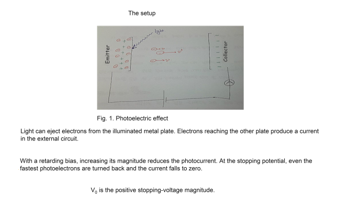
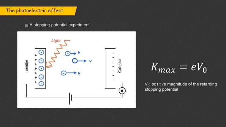
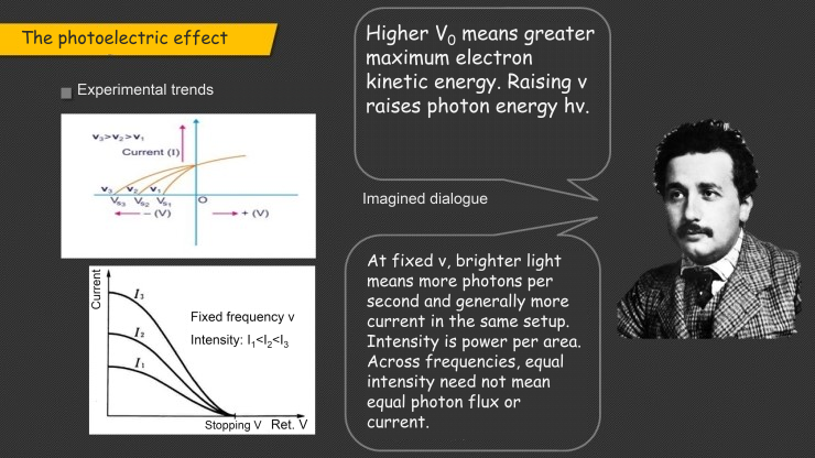
Shine light onto a metal surface, collect the emitted electrons, and measure the current. A voltage that opposes their motion reduces the collected current. At the stopping voltage, even the fastest emitted electrons can no longer reach the collector. Here $V_0$ is the positive magnitude of that retarding voltage, and $e$ is the positive elementary charge:

$$ K_{\max}=eV_0. $$

The relation describes the idealized energy balance used to interpret the experiment. Actual measurements also require attention to the apparatus and contact potentials. MIT’s photoelectric-effect laboratory guide describes this measurement.

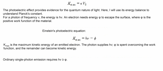
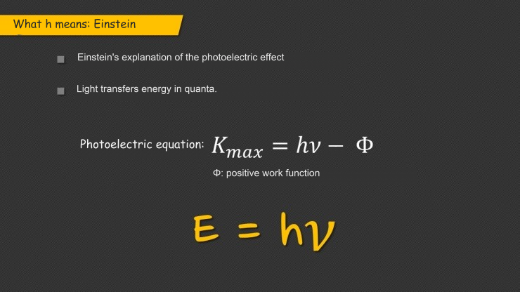
A photon of frequency $\nu$ carries energy $h\nu$. An electron must use some of that energy to escape the metal. If the positive work function is $\Phi$, the largest kinetic energy of an emitted electron is

$$ K_{\max}=h\nu-\Phi. $$

Thus the work function is an energy cost, which explains the minus sign. In the ordinary single-photon model, emission requires $h\nu\geq\Phi$, giving the threshold frequency $\nu_0=\Phi/h$. MIT’s introductory quantum-mechanics lecture notes develop this relation.

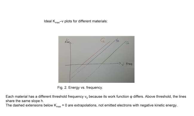
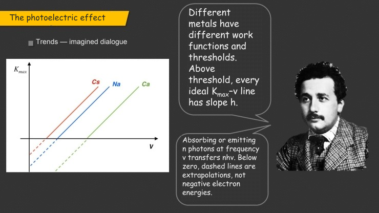
For different metals, the ideal $K_{\max}$ versus $\nu$ graphs have different thresholds but the same slope:

$$ \frac{dK_{\max}}{d\nu}=h. $$

The dashed extensions below the horizontal axis locate the intercept $-\Phi$; they do not represent emitted electrons with negative kinetic energy.

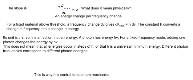
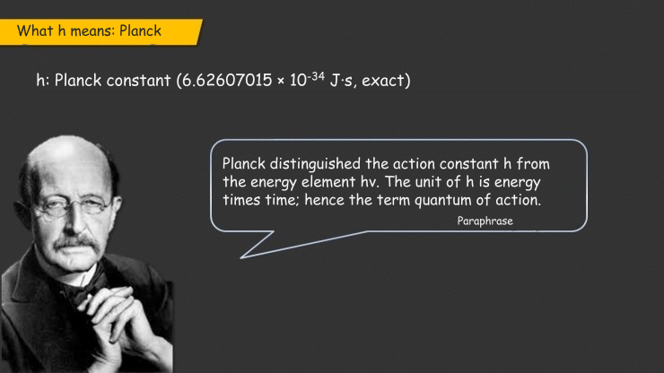
This slope is the point I wanted to emphasize in the report. Increasing frequency by $\Delta\nu$ increases the maximum kinetic energy by $h\Delta\nu$. It does not follow that all energies increase in steps of $h$. Frequency has units of inverse seconds, so the slope has units of joule seconds. Planck’s constant is a quantity of action. The photon energy is $h\nu$, and its value depends on frequency; $h$ alone is not a universal minimum energy.

The route from blackbody radiation to light quanta

The presentation follows the historical thread behind those equations. Einstein’s contribution in 1905 was a theoretical proposal about light quanta and its application to the photoelectric effect. Calling the illustrated apparatus “Einstein’s 1905 experiment,” as the original notes did, confuses the explanation with the experimental work. The Nobel archives’ account of the dual nature of light describes that distinction.

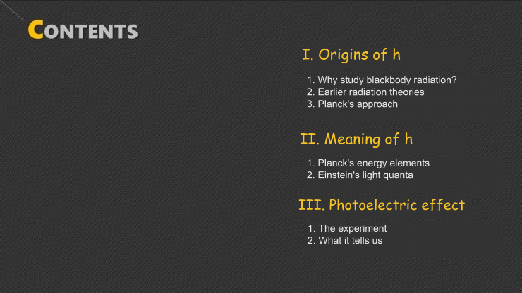
The people and the problem

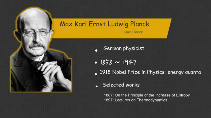
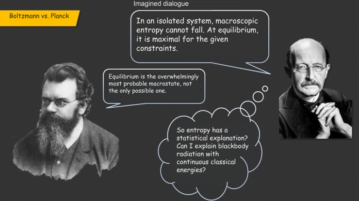
The first slides introduce Max Planck and Ludwig Boltzmann. The cartoon conversation is my way of presenting a conceptual tension: should thermal equilibrium be understood through macroscopic thermodynamic laws or through the statistics of microscopic states? It is a simplified teaching scene, not a transcript of a meeting or evidence of either physicist’s exact thoughts.

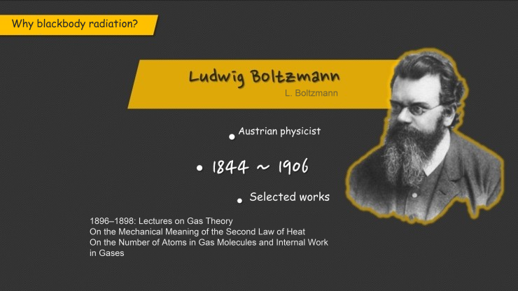
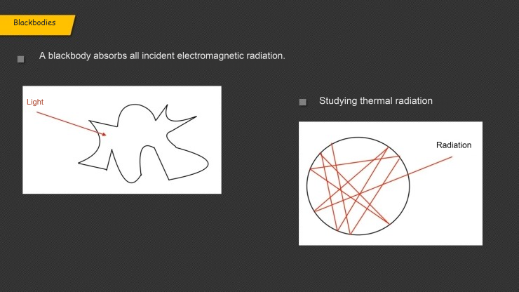
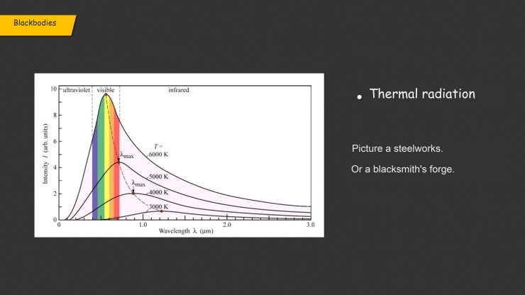
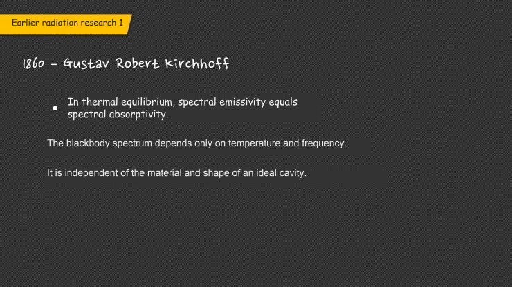
A blackbody absorbs all incident radiation. A small cavity opening can approximate one. At equilibrium, hotter blackbodies emit more power and their wavelength spectra peak at shorter wavelengths. Kirchhoff’s law links emission and absorption at the same wavelength under matching equilibrium conditions. NIST’s manual on blackbody radiation explains these properties.

Three radiation formulas, and two different Wien laws

Wien’s displacement law locates the peak of the spectrum expressed per unit wavelength:

$$ \lambda_{\max}T=b, \qquad b\approx2.898\times10^{-3}\ \mathrm{m\,K} =2898\ \mathrm{\mu m\,K}. $$

The original slide’s value of $2.898\ \mathrm{\mu m\,K}$ was too small by a factor of 1,000. The corrected value agrees with NIST’s physical-constants table.

Wien’s distribution law approximates Planck’s spectrum at short wavelengths. Rayleigh–Jeans approximates it at long wavelengths and fails at short wavelengths. These approximations differ from the displacement law. NIST’s radiation manual distinguishes them.

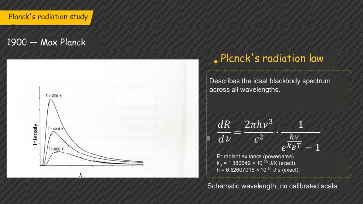
The comparison curves in the next three slides are schematic. Their original numerical wavelength scales were inconsistent with the temperature labels, so the English edition removes those numerical labels. For example, Wien’s displacement law gives a peak near 580 nm at 5,000 K. The sketches illustrate qualitative differences between the formulas, rather than calibrated wavelength measurements.

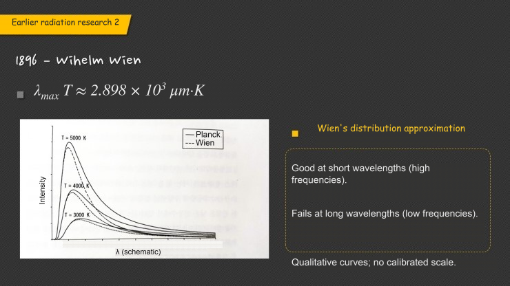
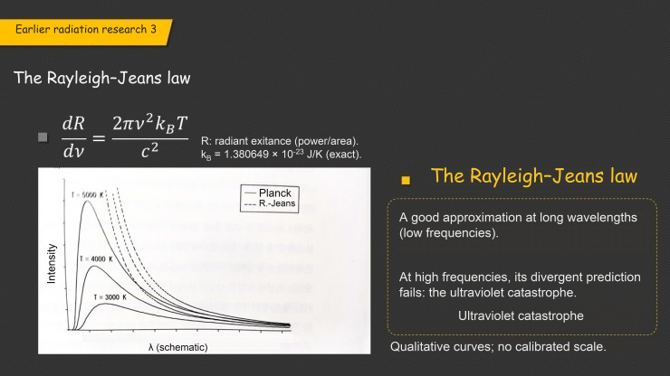
Following the slides, let $dR$ denote the power emitted per unit surface area in a frequency interval $d\nu$. The blackbody spectral radiant exitance in vacuum is

$$ \frac{dR}{d\nu} =\frac{2\pi h\nu^3}{c^2} \frac{1}{\exp\!\left(h\nu/(k_BT)\right)-1}. $$

$c$ is the speed of light; $k_B$ is Boltzmann’s constant. Both the differential and formula use frequency $\nu$. A wavelength spectrum requires the corresponding change of spectral variable. NIST’s radiation manual gives these conventions.

What the constant means

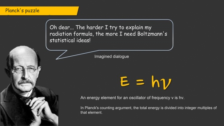
For an oscillator of fixed frequency $\nu$, Planck’s energy elements have size $h\nu$. The corresponding quantum harmonic oscillator has adjacent energy levels separated by $h\nu$; for light, a photon has energy $h\nu$. The frequency must be specified before this becomes a particular energy scale. The slide’s large $E=h\nu$ refers to one energy quantum, rather than every possible total energy. MIT’s quantum-mechanics lecture notes introduce this quantization.

The modern SI fixes these numerical values exactly:

$$ h=6.62607015\times10^{-34}\ \mathrm{J\,s}, \qquad k_B=1.380649\times10^{-23}\ \mathrm{J\,K^{-1}}. $$

The numerical values printed in the original slides are replaced here by the present exact SI values. The unit $\mathrm{J\,s}$ is central to the meaning of $h$: multiplying it by frequency gives energy. These exact values are stated in the BIPM definition of the SI.

Reading the photoelectric graphs

The final slides return to Einstein’s light-quantum explanation and the experiment. Their guiding equation is the energy balance $h\nu=\Phi+K_{\max}$. The experiment probes how light transfers energy to matter; it does not make interference and diffraction disappear. The Nobel archives trace how these different aspects of light were reconciled.

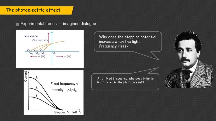
In the ideal single-photon regime, increasing frequency above threshold raises the stopping-voltage magnitude. Increasing intensity at a fixed frequency raises the photon arrival rate and generally the photocurrent, without raising the stopping voltage. When comparing different frequencies, equal optical power does not mean equal photon flux: a beam’s photon rate is its power divided by $h\nu$. MIT’s photoelectric-effect laboratory guide explains the roles of voltage, frequency, and intensity.

The material comparison brings the argument together: changing the metal changes $\Phi$ and the threshold, while the ideal energy–frequency slope remains $h$. It is useful to keep the two roles separate. The work function tells us about the surface; Planck’s constant connects frequency to the energy of a quantum.

That is the path I wanted the presentation to follow: from a problem about heat and radiation to a new way of thinking about light. It is also why I find a small constant in an equation much more interesting once I understand the question that made it necessary.

Sources for the original presentation

The original reference slide lists these Korean-language editions. The titles below are given in English for readability:

1. Kang Ju-sang, Quantum Physics, Cheongmungak, 2004.
2. Jim Baggott, The Quantum Story, Korean translation by Park Byeong-cheol, Banni, 2014.

These are the presentation’s stated reading sources. The primary and institutional references linked in the explanatory text support the scientific corrections in this English edition.