Derivation of the Maxwell Stress Tensor — Appendix

So I was just studying along and got to the Maxwell stress tensor. I absolutely loathe just memorizing it, and my head isn’t that great, so I did it the brute-force way. The cropped steps are below, with the full notebook pages at the end.

What are we actually trying to turn into a tensor?

Start with force per volume

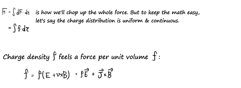
The starting point is the Lorentz force density, not a mysterious matrix:

$$\vec f=\rho\vec E+\vec J\times\vec B,\qquad \vec F=\int_V\vec f\,d\tau.$$

Here $\rho$ is charge per volume and $\vec J$ is current per area. We use SI vacuum-form Maxwell equations with $\varepsilon_0$ and $\mu_0$, and smooth fields where the derivatives are taken. The charge distribution need not be spatially uniform. For charges moving together, $\vec J=\rho\vec v$ gives the form in the first picture.

We want the force written in terms of the fields, so replace the sources using

$$\rho=\varepsilon_0\nabla\cdot\vec E,\qquad \vec J=\frac1{\mu_0}\nabla\times\vec B-\varepsilon_0\frac{\partial\vec E}{\partial t}.$$

Watch the $1/\mu_0$: the red line in the notes has a slip, but the substitution immediately below it uses the right factor.

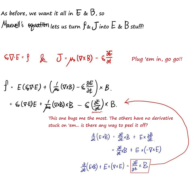
The awkward term is $-\varepsilon_0(\partial\vec E/\partial t)\times\vec B$. Apply the time product rule to $\vec E\times\vec B$, then use Faraday’s law $\partial\vec B/\partial t=-\nabla\times\vec E$. This gives

$$\frac{\partial\vec E}{\partial t}\times\vec B =\frac{\partial}{\partial t}(\vec E\times\vec B)+\vec E\times(\nabla\times\vec E).$$

So one piece is a time derivative of the field’s momentum density. Keep it separate while we tidy the spatial derivatives.

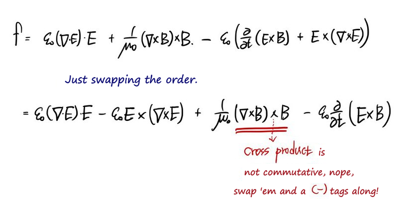
Next, $(\nabla\times\vec B)\times\vec B=-\vec B\times(\nabla\times\vec B)$. Add the zero term $(\nabla\cdot\vec B)\vec B/\mu_0$ and the electric and magnetic expressions have the same shape. Adding zero is doing actual useful work here, heh.

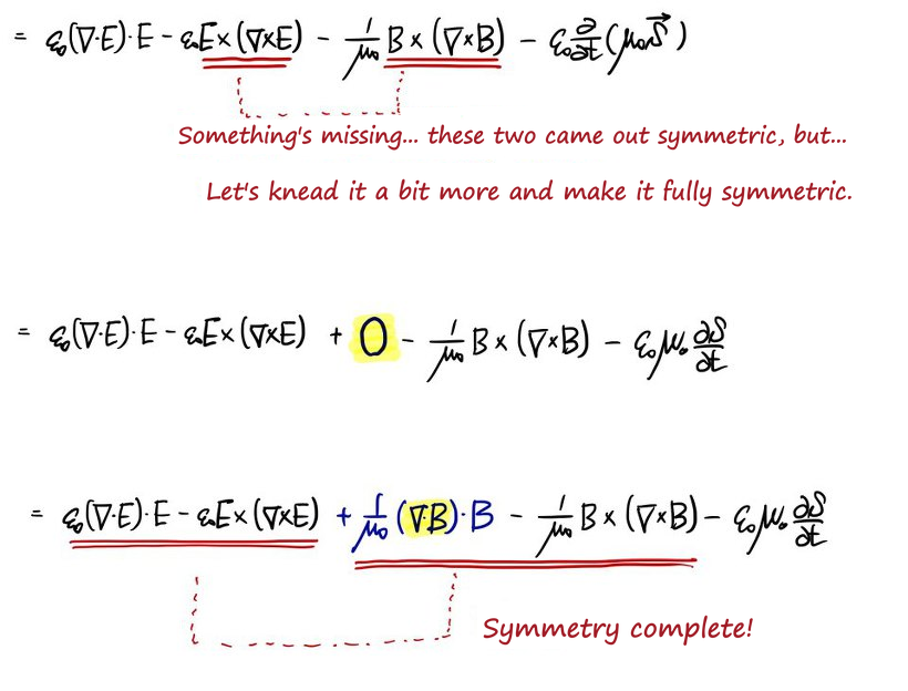
The vector identity that does the heavy lifting

For either field $\vec A$, the product rule says

$$-\vec A\times(\nabla\times\vec A) =(\vec A\cdot\nabla)\vec A-\frac12\nabla(A^2).$$

The last operation is the gradient of a scalar, not a divergence. Also notice the plus sign on $(\vec A\cdot\nabla)\vec A$ after substituting the identity.

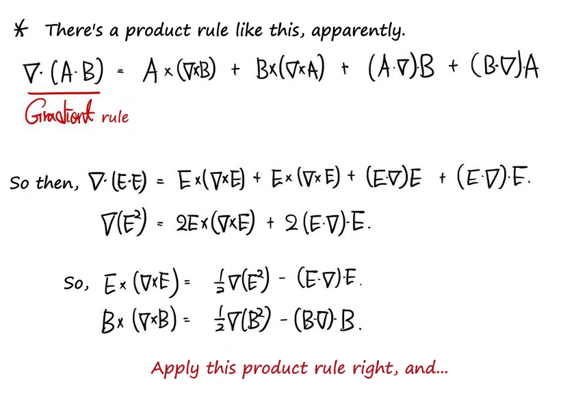
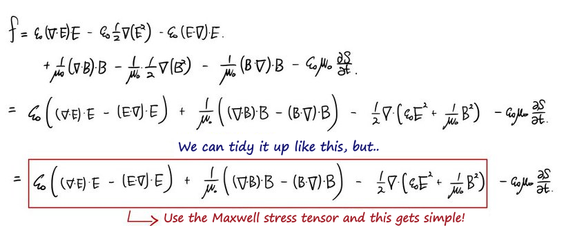
Let $w=(\varepsilon_0E^2+B^2/\mu_0)/2$ and $\vec g=\varepsilon_0\vec E\times\vec B$. The correctly collected force is

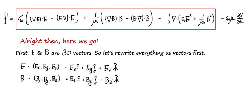
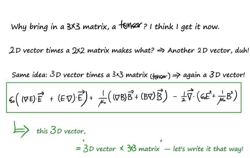
$$\begin{aligned} \vec f={}&\varepsilon_0[(\nabla\cdot\vec E)\vec E+(\vec E\cdot\nabla)\vec E]\\ &+\frac1{\mu_0}[(\nabla\cdot\vec B)\vec B+(\vec B\cdot\nabla)\vec B]\\ &-\nabla w-\frac{\partial\vec g}{\partial t}. \end{aligned}$$

The red box in the old notes accidentally puts minus signs on those directional-derivative terms. Read it using the corrected expression above; the later component calculations and final tensor have the right signs.

What the tensor has to contain

From here the brute-force part begins… ugh! We want to package all the spatial terms as $\nabla\cdot\mathbf T$. The result we’re trying to explain is

$$\begin{aligned} T_{ij}={}&\varepsilon_0\left(E_iE_j-\frac12\delta_{ij}E^2\right)\\ &+\frac1{\mu_0}\left(B_iB_j-\frac12\delta_{ij}B^2\right). \end{aligned}$$

The indices $i,j$ run over $x,y,z$; $\delta_{ij}$ is 1 on the diagonal and zero otherwise. So the field products fill the matrix, and the scalar $w$ is subtracted only from its diagonal entries.

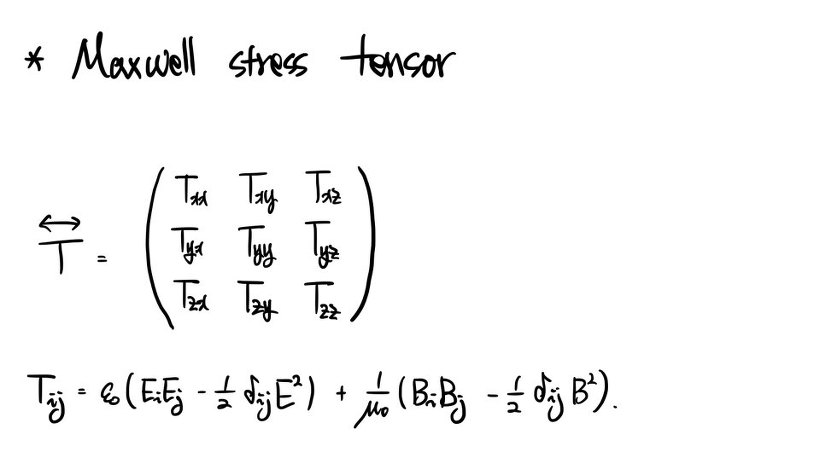
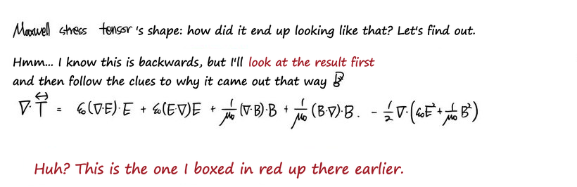
Here is the component check we’re aiming for. I use the convention

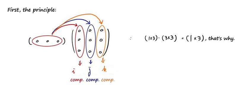
$$(\nabla\cdot\mathbf T)_i=\sum_j\frac{\partial T_{ij}}{\partial x_j}.$$

The tensor is symmetric, $T_{ij}=T_{ji}$, so the transposed-looking row notation in the notes gives the same components. But $\nabla$ is a differential operator acting on the entries, not an ordinary numerical vector multiplying a matrix.

Regroup the product derivatives

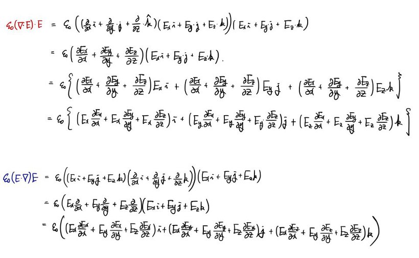
Take the electric part first. The product rule is the whole mechanism:

$$\sum_j\partial_j(E_iE_j) =\sum_j E_j\partial_j E_i+E_i\sum_j\partial_jE_j.$$

Those are exactly the $i$ components of $(\vec E\cdot\nabla)\vec E$ and $(\nabla\cdot\vec E)\vec E$. We haven’t invented a new force; we’ve recognized two terms as the derivative of a product.

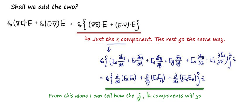
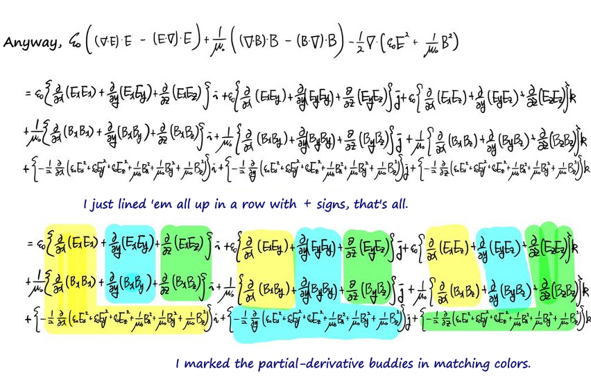
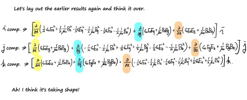
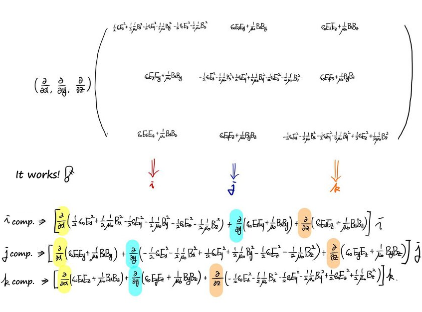
For the $x$ component, for example, those products are $\partial_x(E_x^2)+\partial_y(E_xE_y)+\partial_z(E_xE_z)$. Repeat with $i=y,z$, then do the same with $\vec B/\sqrt{\mu_0}$ in place of $\sqrt{\varepsilon_0}\vec E$. That’s what the next sheet lays out.

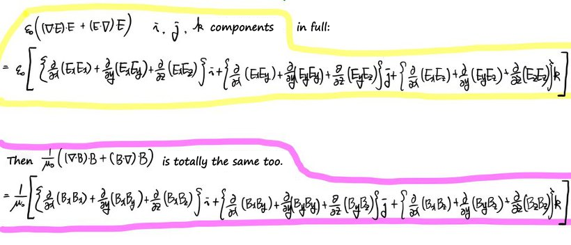
The remaining $-\nabla w$ contributes $-\partial_xw$, $-\partial_yw$, $-\partial_zw$. Equivalently it comes from differentiating $-\delta_{ij}w$ in the tensor — the reason for that diagonal subtraction.

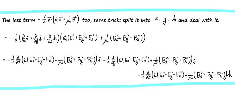
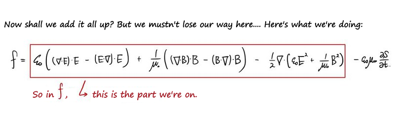
Now match terms by which derivative acts on them. The colored groups below collect $\partial_x$, $\partial_y$ and $\partial_z$, so the matrix entries emerge instead of being guessed.

For the $x$ component, the answer must be $\partial_xT_{xx}+\partial_yT_{xy}+\partial_zT_{xz}$. In particular,

$$T_{xx}=\varepsilon_0E_x^2+\frac{B_x^2}{\mu_0}-w, \qquad T_{xy}=\varepsilon_0E_xE_y+\frac{B_xB_y}{\mu_0}.$$

Only one $-\varepsilon_0E_x^2/2$ belongs inside $-w$; the first expanded line in the picture duplicates it before the next line puts it right.

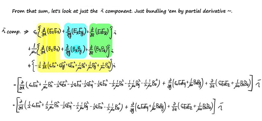
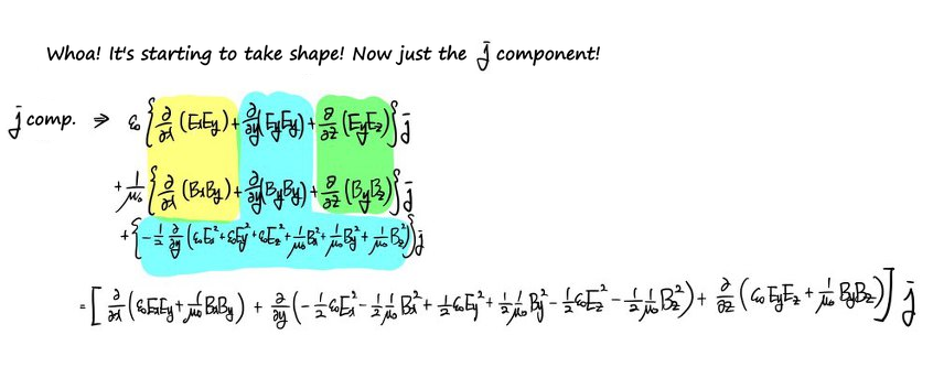
Now each row of the force expression has three spatial derivatives, and each derivative carries one stress entry. That’s why a $3\times3$ array is the natural package — not merely because multiplying compatible matrices happens to give a vector.

Put back the field momentum

We left the time derivative alone, so now the result is

$$\vec f=\nabla\cdot\mathbf T-\frac{\partial\vec g}{\partial t}, \qquad \vec g=\varepsilon_0\vec E\times\vec B=\frac{\vec S}{c^2}.$$

Here $\vec S=\vec E\times\vec B/\mu_0$ and $c^{-2}=\varepsilon_0\mu_0$. This is the same final formula as the notes:

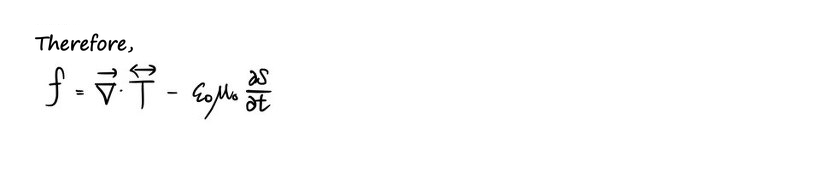
Why the last term? A change in momentum can go into the fields, not only into matter. For a fixed volume, the divergence theorem turns the result into

$$\vec F_{\rm matter}=\oint_{\partial V}\mathbf T\cdot\hat n\,da -\frac{d}{dt}\int_V\vec g\,d\tau.$$

The outward normal is $\hat n$. The surface stress gives the mechanical force only after we subtract the rate at which field momentum inside the volume is changing. In a static situation, that time derivative vanishes.

Two checks I like: every $T_{ij}$ has units of energy per volume, the same as force per area. And for uniform static $\vec E=E_0\hat x$, $\vec B=0$, the diagonal entries are $(+w,-w,-w)$ with $w=\varepsilon_0E_0^2/2$. They’re nonzero, but their divergence is zero: a uniform stress is not a nonzero local force density everywhere.

Full notebook pages

These are the same steps in their original page layout, kept for cross-checking the cropped equations. The slips noted above and in the Heads-up still belong to the original pages.

---

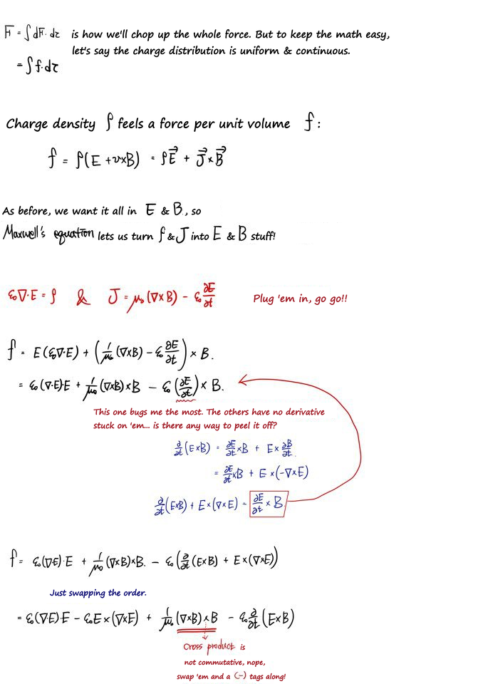
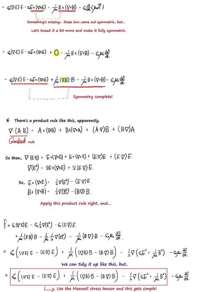
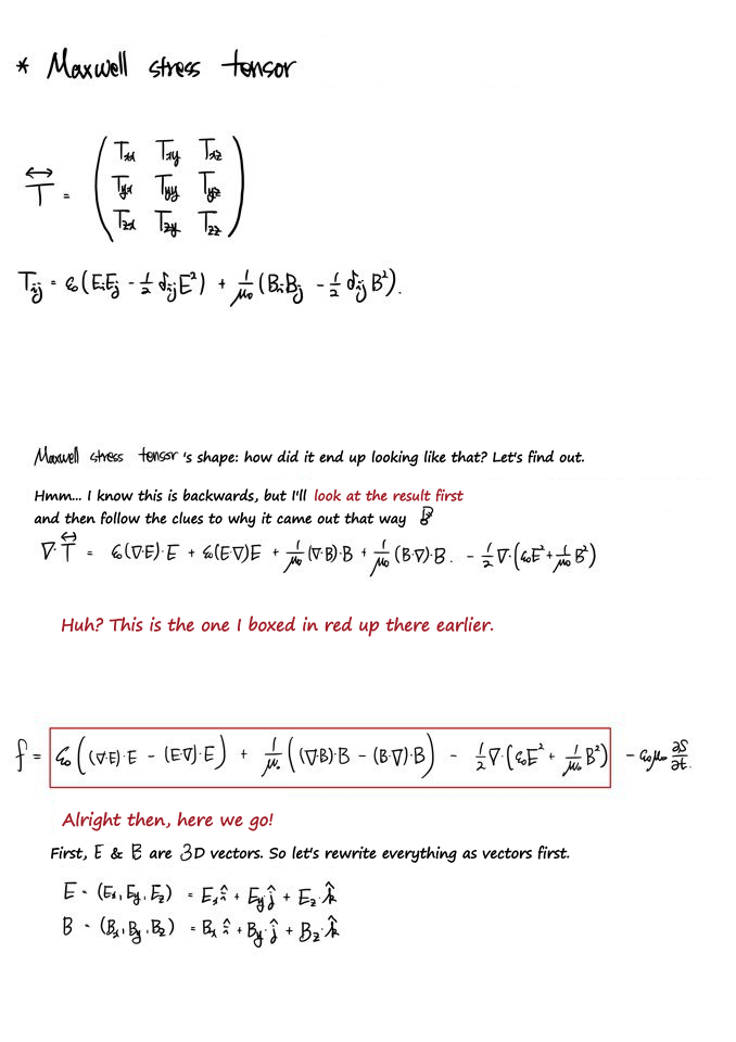
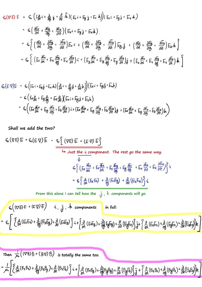
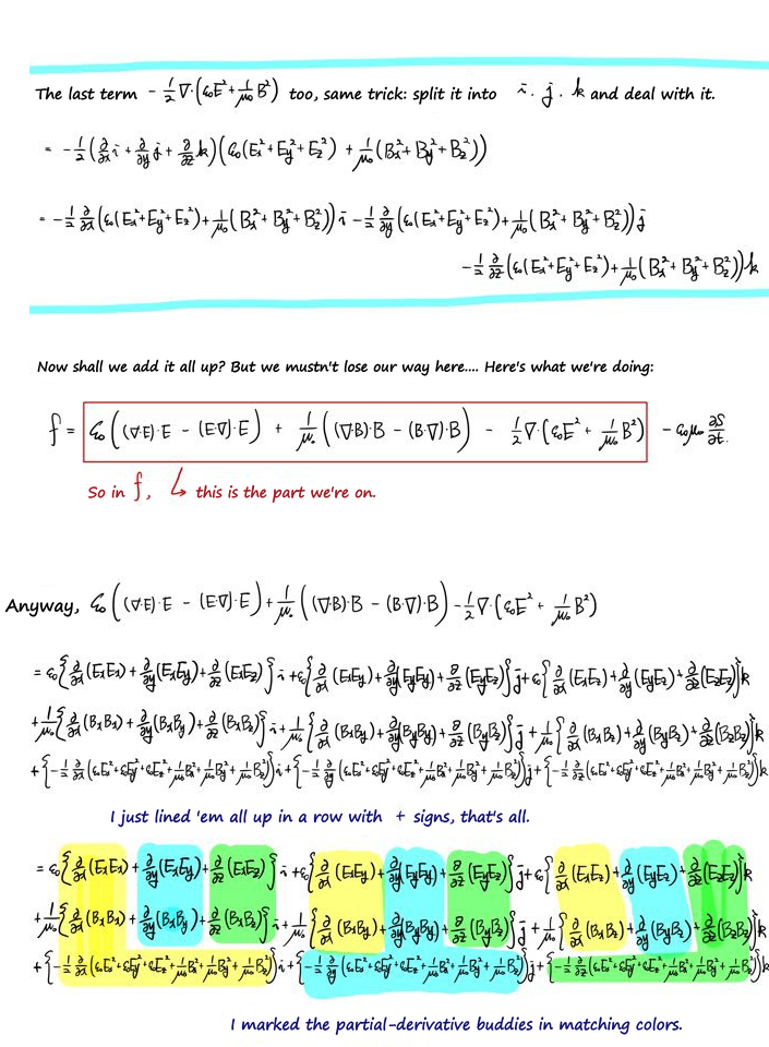
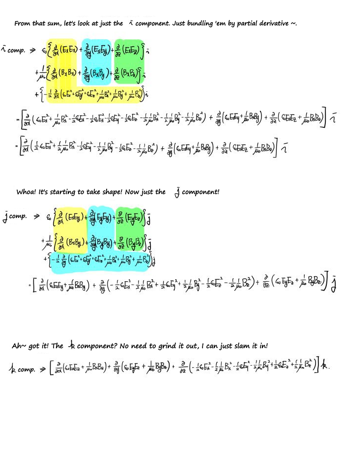
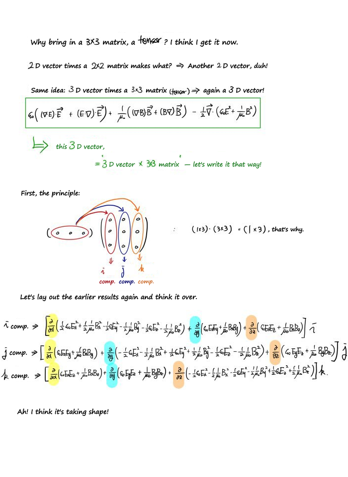
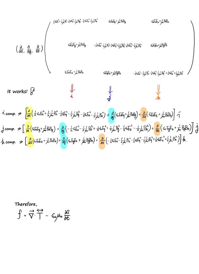
Heads-up. The figures here are the original notes, slips and all. A few things to watch for:

• In the first picture, $\vec{F} = \int d\vec{F}\cdot d\tau$ should read $\vec{F} = \int d\vec{F} = \int \vec{f}\,d\tau$ (the line below it has it right).
• The red Ampère–Maxwell line should read $\vec{J} = \frac{1}{\mu_0}(\nabla\times\vec{B}) - \varepsilon_0\frac{\partial\vec{E}}{\partial t}$, with the $\frac{1}{\mu_0}$ that the next line uses.
• Wherever $\nabla\cdot$ stands in front of a scalar ($\nabla\cdot(\vec{A}\cdot\vec{B})$, $\nabla\cdot(\vec{E}\cdot\vec{E})$, $\nabla\cdot(\varepsilon_0E^2 + B^2/\mu_0)$), read the gradient $\nabla$.
• Putting $\vec{E}\times(\nabla\times\vec{E}) = \frac{1}{2}\nabla(E^2) - (\vec{E}\cdot\nabla)\vec{E}$ in gives $+\varepsilon_0(\vec{E}\cdot\nabla)\vec{E}$ and $+\frac{1}{\mu_0}(\vec{B}\cdot\nabla)\vec{B}$, so the red box (and its copies further down) should read $\vec{f} = \varepsilon_0[(\nabla\cdot\vec{E})\vec{E} + (\vec{E}\cdot\nabla)\vec{E}] + \frac{1}{\mu_0}[(\nabla\cdot\vec{B})\vec{B} + (\vec{B}\cdot\nabla)\vec{B}] - \frac{1}{2}\nabla\left(\varepsilon_0E^2 + \frac{1}{\mu_0}B^2\right) - \varepsilon_0\mu_0\frac{\partial\vec{S}}{\partial t}$. The divergence of the stress tensor and the final $\vec{f} = \nabla\cdot\overleftrightarrow{T} - \varepsilon_0\mu_0\frac{\partial\vec{S}}{\partial t}$ are right.
• In the first line of the $\hat{i}$ component, $-\frac{1}{2}\varepsilon_0E_x^2$ appears twice; it belongs there once, as the next line shows.