Chapter 2 & 3 Practice Problems

Prob 2.6 — one demand curve, three elasticities

Let’s start by separating two things that look similar on a graph: the slope of demand and its elasticity.

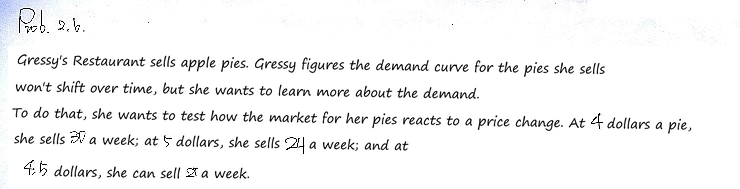
Here the price changes while the demand curve is assumed to stay put. The three observations are $(P,Q)=(4,30),(4.5,27),(5,24)$. Each half-dollar increase costs three sales, so $dQ/dP=-6$.

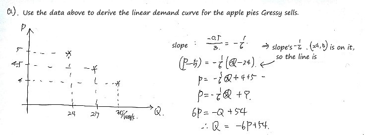
Put that slope through any observed point: $Q=54-6P$, or $P=9-Q/6$. Check the middle observation: $54-6(4.5)=27$. The graph puts price vertically, so its drawn slope is $dP/dQ=-1/6$, the reciprocal of the derivative we use next.

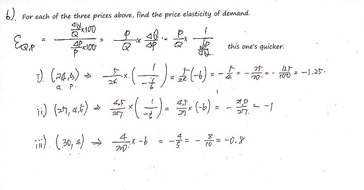
Point elasticity is $E_{Q,P}=(dQ/dP)(P/Q)=-6P/Q$. At prices 5, 4.5 and 4 it is respectively −1.25, −1 and −0.8. Same straight line, same slope — but different percentage responses because the starting price and quantity change. At the middle point demand is unit elastic; it isn’t equally elastic everywhere on the line.

Prob 2.13 — what can elastic demand tell us?

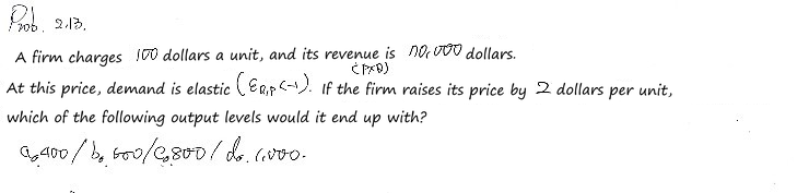
Revenue divided by price gives the starting quantity: $70{,}000/100=700$. A rise of 2 on a price of 100 is a 2% increase. With elastic demand, the local percentage fall in quantity is larger than 2%.

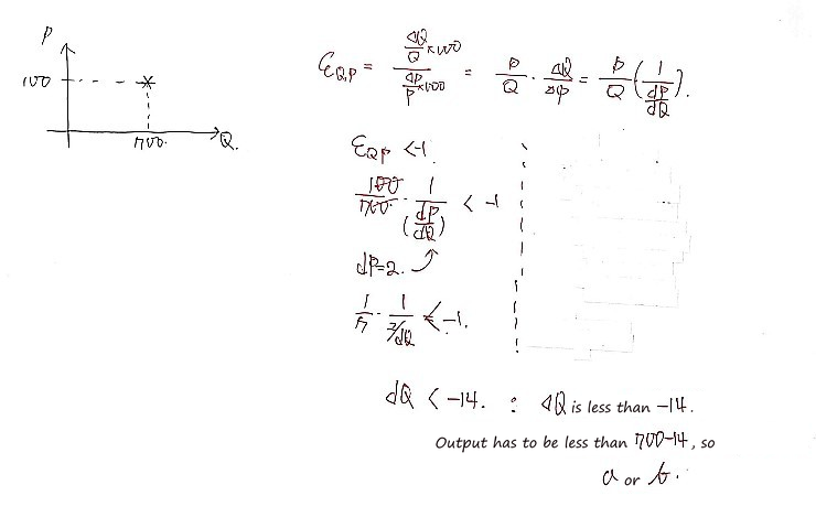
Using the small-change approximation, $dQ/dP<-7$, so a 2-dollar rise suggests a quantity fall greater than 14, to below about 686. That leaves choices a or b on the sheet. It doesn’t pick one of those two. We would need more of the demand curve to determine the exact finite change; point elasticity at the starting price alone is not enough.

Prob 2.14 — spending gives us a clue

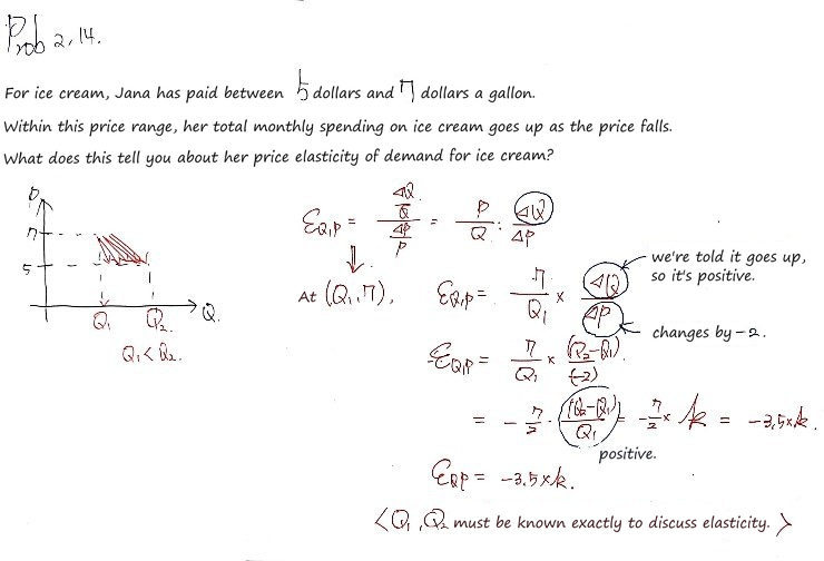
My last handwritten sentence is too pessimistic: we don’t need both quantities exactly. Spending rises when price falls from 7 to 5, so $5Q_2>7Q_1$, which means $Q_2>1.4Q_1$. Quantity rises by more than 40%.

With the picture’s starting-value percentage convention, $E=-3.5k$ and $k=(Q_2-Q_1)/Q_1>0.4$, hence $E<-1.4$. The observed change is price elastic. This classifies the response over that price change; it does not reconstruct the demand curve’s point elasticity at every intervening price.

Prob 2.16 — golf balls, rubber and titanium

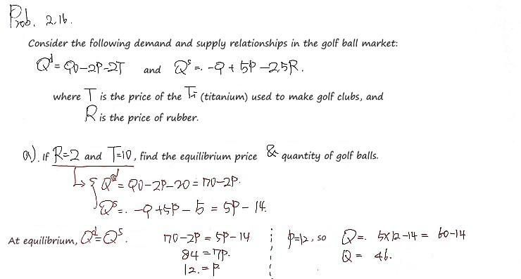
Set the given input prices first: $R=2$ and $T=10$. Then $Q^d=70-2P$ and $Q^s=5P-14$. Equilibrium means the two quantities agree: $70-2P=5P-14$, so P = 12 and Q = 46. Both equations give 46 — a quick way to catch a transcription mistake.

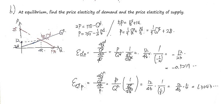
Now use the derivatives, not the slopes of the inverse curves: demand has $dQ^d/dP=-2$, supply has $dQ^s/dP=5$. At the same equilibrium, their elasticities are $-2(12/46)=-12/23\approx-0.522$ and $5(12/46)=30/23\approx1.304$.

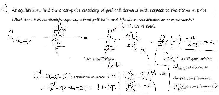
For the cross-price elasticity, change the titanium price while holding the golf-ball price fixed. Here $\partial Q^d/\partial T=-2$, so $E_{Q,T}=-2(10/46)=-10/23\approx-0.435$. More expensive titanium raises the cost of golf clubs and reduces demand for balls: the sign says complements in this model. The handwritten intermediate price 13 should be 12; the final derivative and elasticity are unchanged.

Marginal utility and indifference curves

Prob 3.7 — more utility, but smaller extra gains

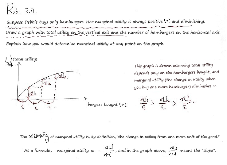
Positive marginal utility makes total utility rise as Debbie gets more hamburgers. Diminishing marginal utility makes that rise flatten out. The marginal utility at a point is the slope of the total-utility curve, not its height: $MU=dU/dQ$.

Another utility curve: one good and one bad

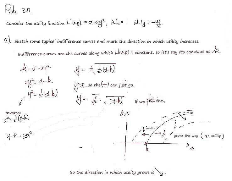
This one is different: $U=x-2y^2$ has $MU_x=1$ but $MU_y=-4y$. With nonnegative quantities, more x helps and more y hurts. Holding utility at k gives $y=\sqrt{(x-k)/2}$, with $x\ge k$. The curves slope upwards because extra x must compensate for extra y; utility improves towards more x and less y.

Prob 3.8 — don’t keep the wrong half of the parabola

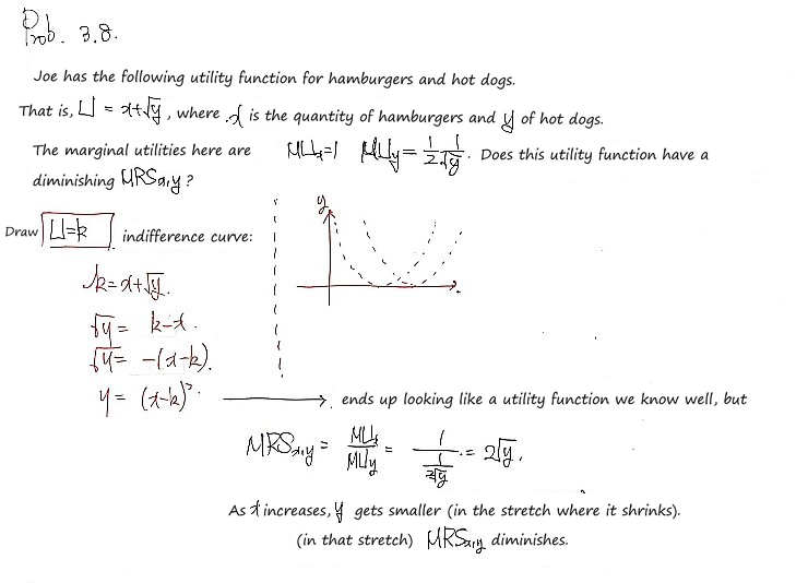
For $U=x+\sqrt y=k$, we have $\sqrt y=k-x$. Squaring gives $y=(k-x)^2$, but only where $0\le x\le k$. The rising half would make $k-x$ negative and cannot satisfy the original equation.

The positive MRS is $MU_x/MU_y=2\sqrt y$. Along the valid indifference curve, x rises and y falls, so this MRS diminishes. Keep the signs straight: the actual curve slope is minus that ratio.

Prob 3.12 — Bond wants the recipe, not extra vodka

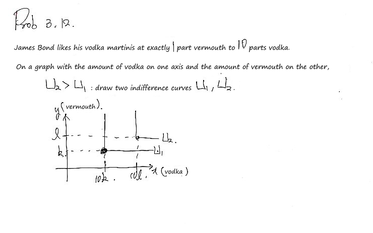
The useful combination is one part vermouth with ten parts vodka. With vodka on the horizontal axis, the corners lie on $x=10y$. Extra vodka alone doesn’t improve the drink when vermouth is the bottleneck, and vice versa — hence the flat and vertical arms. More complete recipes move the corner outward to a higher indifference curve.

Prob 3.13 — three different relationships

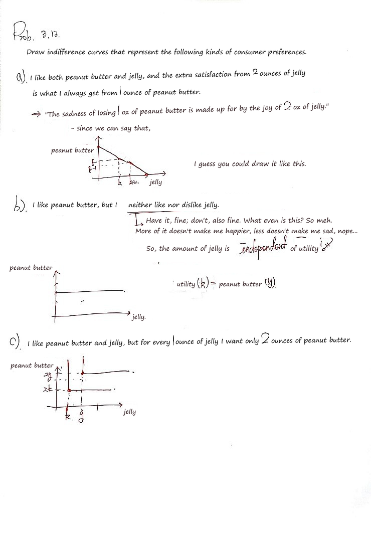
In (a), two ounces of jelly replace one ounce of peanut butter. With jelly horizontally and peanut butter vertically, the straight-line slope is $-1/2$. In (b), jelly is neutral: moving horizontally changes nothing, so the curves are horizontal. In (c), the ingredients are needed together in fixed proportions, two units of peanut butter per unit of jelly; the L-shaped corners lie on $y=2x$. The shapes tell us whether substitution is possible, irrelevant, or useless beyond the recipe.

Prob 3.14 — an increasing MRS

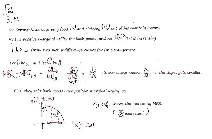
Both goods have positive marginal utility, so the curves still slope down. But this time MRS increases as we move right along a curve. Since $dy/dx=-MRS$, the slope becomes more negative: the curve gets steeper rather than flatter. That’s why these curves bow outward. Don’t lose the minus sign in the handwritten middle step; it is what connects an increasing positive MRS to a falling signed slope.

---

Heads-up. The figures here are the original notes, slips and all. A few things to watch for:

• In Prob 2.14, the elasticity can be pinned down without knowing $Q_1$ and $Q_2$: spending rises as the price falls from 7 to 5, so $5Q_2 \gt 7Q_1$, $k = \frac{Q_2 - Q_1}{Q_1} \gt 0.4$ and $E_{Q,P} = -3.5k \lt -1.4$. Her demand for ice cream is price elastic in that range.
• In Prob 3.14, along an indifference curve $\frac{MU_x}{MU_y} = -\frac{dy}{dx}$, with a minus sign. The conclusion stands: an increasing MRS means the slope $\frac{dy}{dx}$ keeps falling, so the indifference curves bow outward.
• In Prob 2.16 c), the equilibrium price is 12, not the handwritten 13. Holding that price fixed, Qᵈ = 90 − 24 − 2T = 66 − 2T; the derivative −2 and final elasticity −10/23 are unchanged.
• In Prob 3.8, y = (k − x)² represents the indifference curve only where 0 ≤ x ≤ k, since √y = k − x must be nonnegative. The rising half is not part of it.
• Prob 2.13 uses a small-price-change elasticity approximation: at P = 100, Q = 700 and elasticity below −1 imply dQ/dP < −7, so a 2-dollar increase suggests a drop greater than 14. Point elasticity alone does not fix an exact finite change without the demand curve.