Practice Problems: Chapter 20

Prob 20.1

At high temperature, that is, if , show that the partition function of a simple harmonic oscillator is approximately . Then find $U$, $C$, $F$ and $S$ at high temperature.

Solve the same problem for the rotational energy levels of a diatomic molecule too, in the high-temperature limit where .

The routine in these problems is: count the energy states first, then differentiate $\ln Z$. Here $\beta=1/(k_BT)$, $F=-k_BT\ln Z$, $U=-\partial_\beta\ln Z$, and $S=(U-F)/T$. We’ll keep the oscillator frequency and the rotor’s moment of inertia fixed.

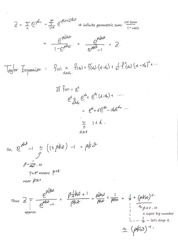
For the oscillator, the exact sum is $Z=[2\sinh(x/2)]^{-1}$ with $x=\beta\hbar\omega$. High temperature means $x\ll1$, so its leading term is $1/x$. This gives $U\approx k_BT$ and $C\approx k_B$ for one oscillator, together with $F\approx k_BT\ln x$ and $S\approx k_B(1-\ln x)$. Those are high-temperature results; we shouldn’t extend that entropy approximation down to zero temperature.

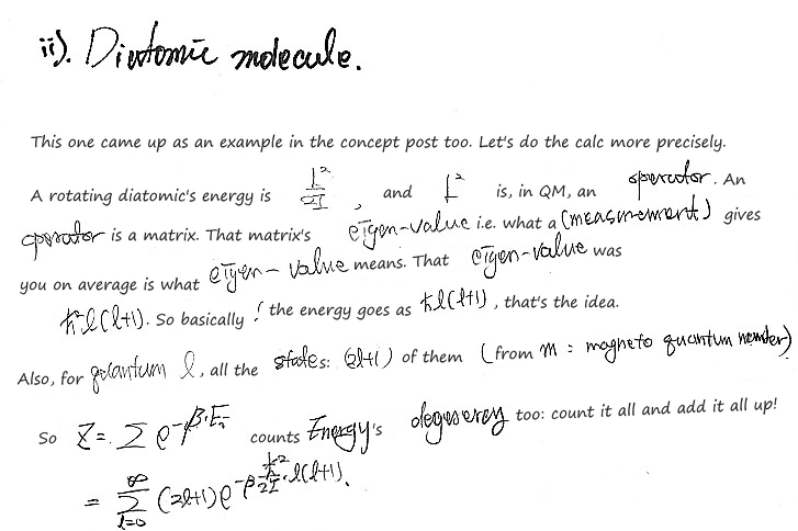
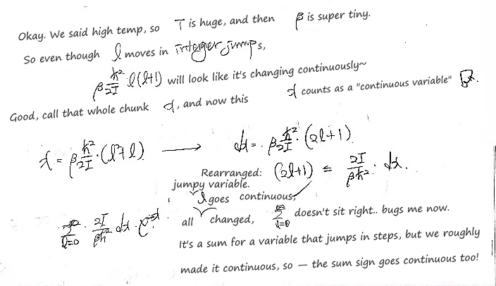
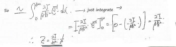
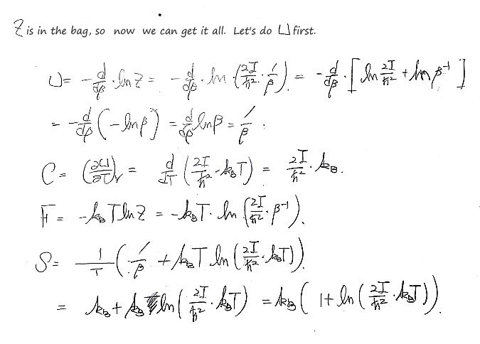
For the rotor, $E_l=\hbar^2l(l+1)/(2I)$ and each $l$ has $2l+1$ states. The eigenvalue is a possible measurement result, not generally an average. When $k_BT\gg\hbar^2/(2I)$, many levels contribute and the sum is well approximated by the integral on the sheets:

$$ Z\approx\frac{2Ik_BT}{\hbar^2},\qquad U\approx k_BT,\qquad C\approx k_B. $$

Notice that the constant $2I/\hbar^2$ drops out when we differentiate $\ln Z$. It belongs in $Z$, $F$ and $S$, but not as an extra factor in $C$. The heat-capacity line in the last rotor sheet is a slip.

Prob 20.2

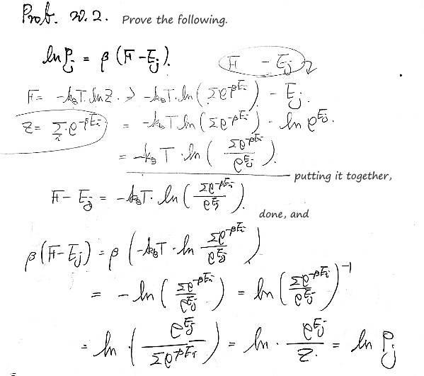
Start straight from the canonical probability $P_j=e^{-\beta E_j}/Z$. Its logarithm is $\ln P_j=-\beta E_j-\ln Z$. Since $\ln Z=-\beta F$, we immediately get

$$ \ln P_j=\beta(F-E_j). $$

The negative exponent matters: higher-energy states should have lower probability at positive temperature. Some intermediate exponents on the sheet lose that sign; use the canonical probability above.

Prob 20.3

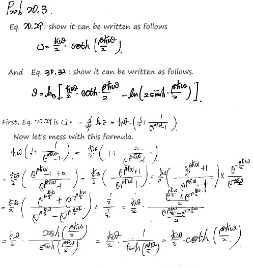
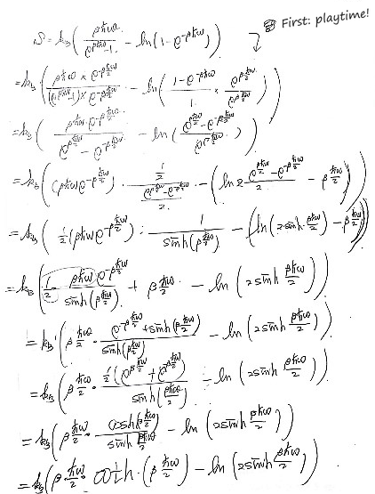
This time we keep the exact oscillator result. Set $x=\beta\hbar\omega$ and write the exponentials as hyperbolic functions:

$$ U=\frac{\hbar\omega}{2}\coth\frac{x}{2},\qquad \frac{S}{k_B}=\frac{x}{2}\coth\frac{x}{2} -\ln\!\left(2\sinh\frac{x}{2}\right). $$

The factor $x/2$ in the entropy is dimensionless. That’s a useful check on the missing $\beta$ in the problem statement. At low temperature $U$ tends to $\hbar\omega/2$ while $S$ tends to zero; at high temperature the formulas return the results of 20.1.

Prob 20.4

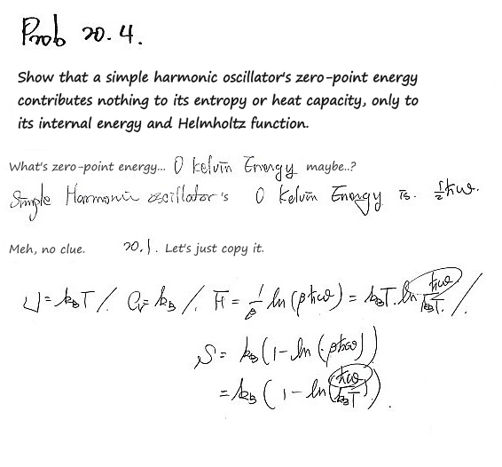
The copied high-temperature formulas don’t by themselves prove the claim. Here’s the short way to see it. Add a constant $E_0=\hbar\omega/2$ to every oscillator level. Then

$$ Z'=e^{-\beta E_0}Z,\qquad U'=U+E_0,\qquad F'=F+E_0. $$

The two shifts cancel in $S=(U-F)/T$, and differentiating the constant shift in $U$ gives zero. So $S'=S$ and $C'=C$. The zero-point energy changes the energy reference, not the relative probabilities of the levels. This argument works at any temperature, with $\omega$ held fixed.

Prob 20.5

Here spin $s=1/2$ has two projections $m_s=\pm1/2$; spin itself isn’t negative. In the model used by this problem, the two energies are $\pm\mu_BB$. We sum their Boltzmann factors, then take the $N$th power because the spins don’t interact.

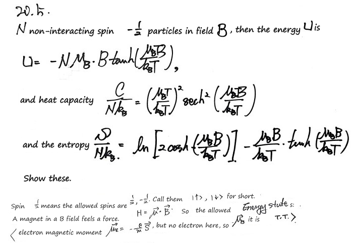
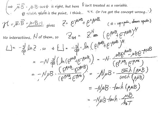
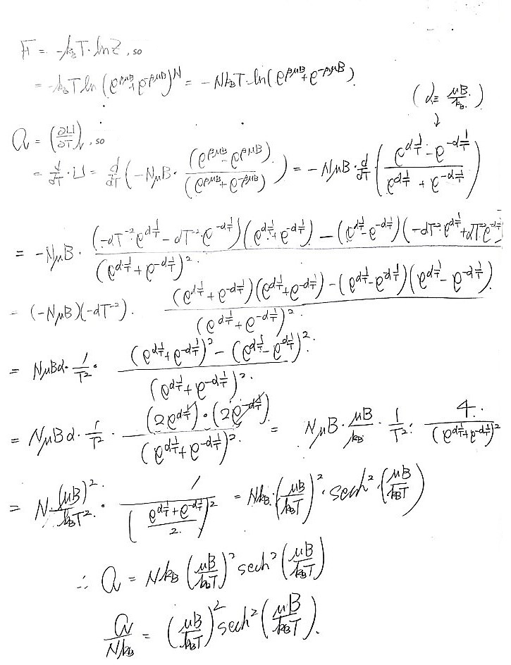
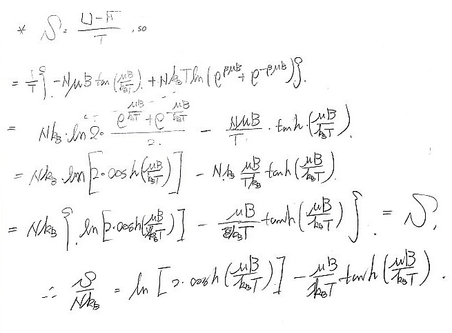
With $x=\mu_BB/(k_BT)$, the one-spin sum is $z=2\cosh x$ and $Z=z^N$. The results can be kept together as

$$ U=-N\mu_BB\tanh x,\qquad C_B=Nk_Bx^2\operatorname{sech}^2x, $$$$ \frac{S}{Nk_B}=\ln(2\cosh x)-x\tanh x. $$

The derivative for $C_B$ holds the field fixed. Both $B$ factors in $x^2$ are needed, despite the typo in the statement. For a nonzero field, cooling favors the lower level and $S\to0$; at high temperature the two levels become equally likely and $S\to Nk_B\ln2$.

Prob 20.6

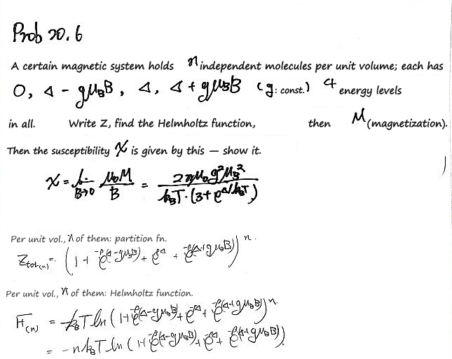
Now there are four levels, and $n$ means molecules per unit volume. Let’s use a lower-case $f$ for free energy per unit volume so that we don’t accidentally multiply by $n$ twice. For one molecule, the level sum is

$$ z=1+e^{-\beta\Delta}[1+2\cosh y], \qquad y=\beta g\mu_BB. $$

Every term is $e^{-\beta E}$ for one of the four listed energies. In a sample of volume $V$, $Z=z^{nV}$ and $f=F/V=-nk_BT\ln z$.

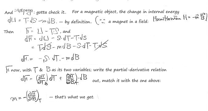
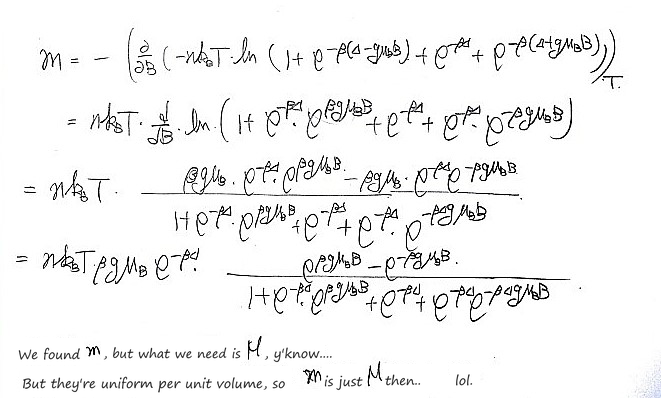
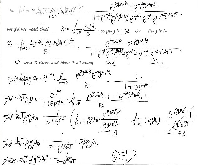
The derivative of that free-energy density is already the magnetization:

$$ M=-\left(\frac{\partial f}{\partial B}\right)_T =\frac{2ng\mu_Be^{-\beta\Delta}\sinh y}{z}. $$

For a weak field, $\sinh y\approx y$ and $z\to1+3e^{-\beta\Delta}$. Dividing by $B$ therefore leaves a finite slope,

$$ \chi=\lim_{B\to0}\frac{\mu_0M}{B} =\frac{2n\mu_0g^2\mu_B^2} {k_BT[3+e^{\Delta/(k_BT)}]}. $$

There is only one density factor $n$. The extra one in the final sheet comes from treating a density as though it were a single molecule’s moment.

Prob 20.7

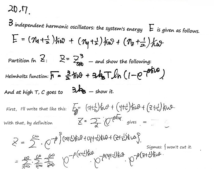
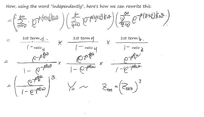
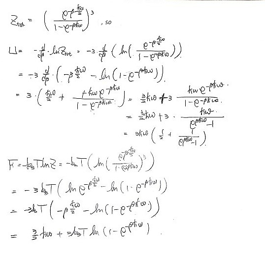
Independence is doing the work here: the energy is a sum, so each Boltzmann factor splits into three factors and the three sums can be done separately. Thus $Z=z^3$, and $\ln Z=3\ln z$ makes $U$ and $F$ three times their one-oscillator values.

For the requested heat capacity, differentiate the energy with $\omega$ fixed. If $x=\beta\hbar\omega$,

$$ C=3k_B\frac{x^2e^x}{(e^x-1)^2}\ \longrightarrow\ 3k_B \quad(x\to0). $$

Each independent oscillator contributes $k_B$ in the high-temperature limit. The constant total zero-point energy $3\hbar\omega/2$ contributes nothing to this derivative, just as in 20.4.

---

Heads-up. The figures here are the original notes, slips and all. A few things to watch for:

• For the rotating diatomic molecule, the energy levels are $E_l = \frac{\hbar^2 l(l+1)}{2I}$ ($\hat{L}^2$ has the eigenvalues $\hbar^2 l(l+1)$), not $\hbar l(l+1)$; the sum at the bottom of that sheet has it right.
• The rotor’s heat capacity comes from $U = k_BT$: $C = \frac{dU}{dT} = k_B$. The sheet differentiates the factor of $Z$ instead and gets $\frac{2I}{\hbar^2}k_B$; $F$ and $S$ are right.
• In Prob 20.2, $E_j = -k_BT\ln e^{-\beta E_j}$, so every $e^{E_j}$ in the steps is $e^{-\beta E_j}$ and $P_j = \frac{e^{-\beta E_j}}{Z}$; the result $\ln P_j = \beta(F - E_j)$ is right.
• In Prob 20.3, the second formula is Eq. 20.32 (not 30.32), and its first term carries the $\beta$: $S = k_B\left[\frac{\beta\hbar\omega}{2}\coth\frac{\beta\hbar\omega}{2} - \ln\left(2\sinh\frac{\beta\hbar\omega}{2}\right)\right]$, as the derivation ends.
• Prob 20.4 is not worked on its sheet (it copies the results of 20.1). The zero-point energy multiplies $Z$ by $e^{-\beta\hbar\omega/2}$, which adds $\frac{\hbar\omega}{2}$ to $U$ and to $F$ and cancels out of $S = \frac{U - F}{T}$ and of $C = \frac{\partial U}{\partial T}$.
• In Prob 20.5, the heat capacity is $\frac{C}{Nk_B} = \left(\frac{\mu_BB}{k_BT}\right)^2\operatorname{sech}^2\frac{\mu_BB}{k_BT}$ (the statement has $\mu_BT$ on top). In Prob 20.6, the last term of the denominator is $e^{-\beta\Delta}e^{-\beta g\mu_BB}$ (no second $\Delta$), and the $m$ from the Helmholtz function of all $n$ molecules in unit volume already is $M$ (not $nm$); neither changes $\chi$, which is right.
• An eigenvalue is a possible measurement result, not generally the average of repeated measurements. For an angular-momentum eigenstate, L² has the definite value ℏ²l(l+1).
• For spin-½, the projections are $m_s=\pm1/2$; the spin quantum number is $s=1/2$. The magnetic interaction is $H=-\boldsymbol\mu\cdot\mathbf B$. The two levels are still $\pm\mu_BB$, so the partition function and final thermodynamic results here are unchanged. The heat capacity is evaluated at fixed field.