Practice Problems: Chapter 29

Chapter 29 was about the Fermi-Dirac & Bose-Einstein distributions.

So why did the post order suddenly jump to Chap 29?

That was just the order I covered the concepts in. The reason is, to derive Stefan-Boltzmann in Chap 23, this is how it had to be done…. (It would have been nice if the book’s order had been this way too, but) I switched the post order for a bit.

Anyway, since I’m only uploading the problems I solved with certainty, it’s a shame there aren’t answers to every problem. Please just use it for reference, and corrections are always welcome!!

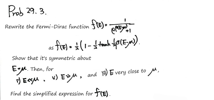
Prob 29.3

Let’s keep one quantity in view: $x=\beta(E-\mu)$, with $\beta=1/(k_BT)$. The distribution tells us the mean occupation of one state, so its value is between zero and one. At $E=\mu$, it is exactly $1/2$.

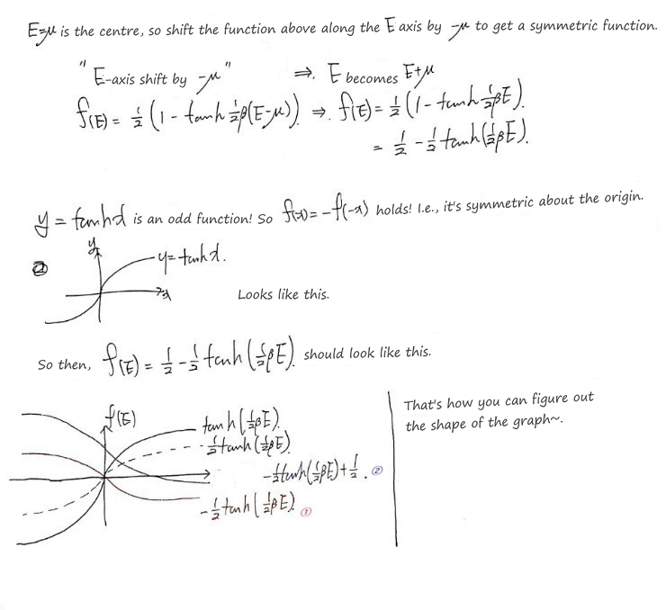
The useful identity is

$$ f(E)=\frac12\left[1-\tanh\!\left(\frac{\beta(E-\mu)}2\right)\right]. $$

Shift the center of the graph to $(\mu,1/2)$ and the remaining tanh is odd. That’s point symmetry, which we can check without drawing anything: $f(\mu+\delta)+f(\mu-\delta)=1$. The extra $1/2$ inside the brackets on the first sheet is a slip; the formula above is the one to use.

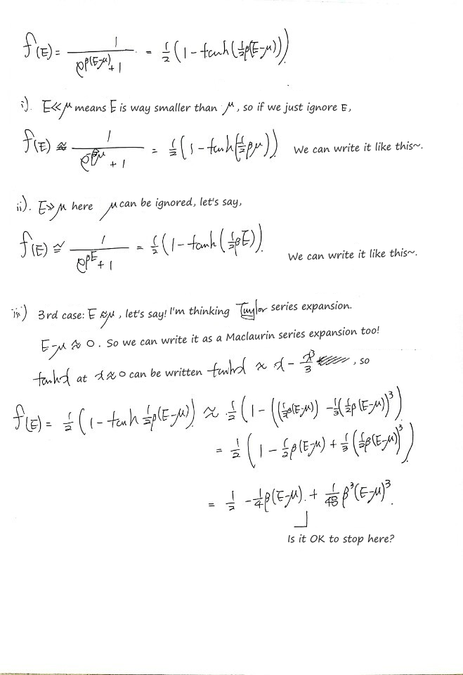
For the limits, compare the energy difference with $k_BT$. If $E-\mu\gg k_BT$, the exponential dominates and $f\approx e^{-\beta(E-\mu)}$. If $\mu-E\gg k_BT$, the state is almost full: $f\approx1-e^{\beta(E-\mu)}$. We keep both $E$ and $\mu$ in those exponents.

Right near the center, $|E-\mu|\ll k_BT$, the expansion on the sheet gives

$$ f(E)\approx\frac12-\frac{\beta(E-\mu)}4 +\frac{\beta^3(E-\mu)^3}{48}. $$

The negative linear term is a quick check: as energy increases through $\mu$, the occupation should fall.

Prob 29.6

(a) Fermions

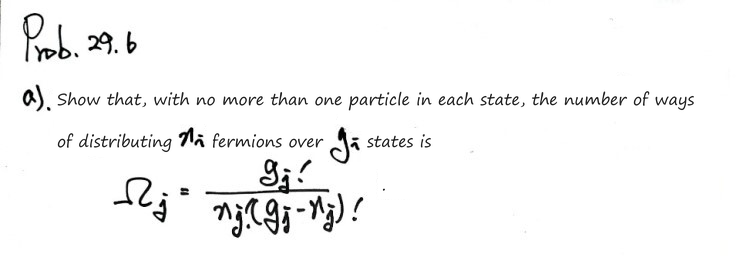
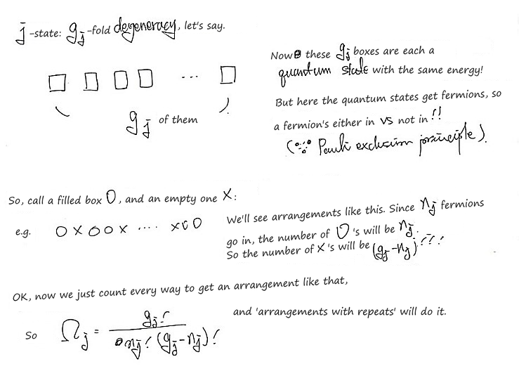
Here $g_j$ is the number of distinct single-particle states with energy $E_j$, and $n_j$ is how many particles occupy that group. The particles aren’t labeled. For fermions we only choose which $n_j$ of the $g_j$ states are filled:

$$ \Omega_j=\binom{g_j}{n_j},\qquad 0\le n_j\le g_j. $$

That’s why swapping two particles doesn’t produce an extra arrangement.

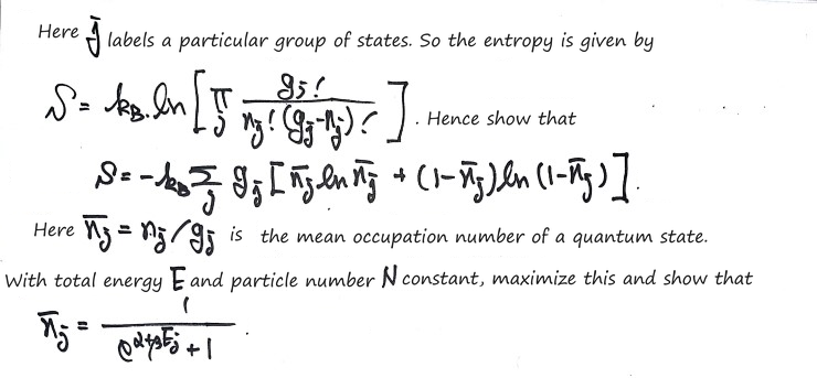
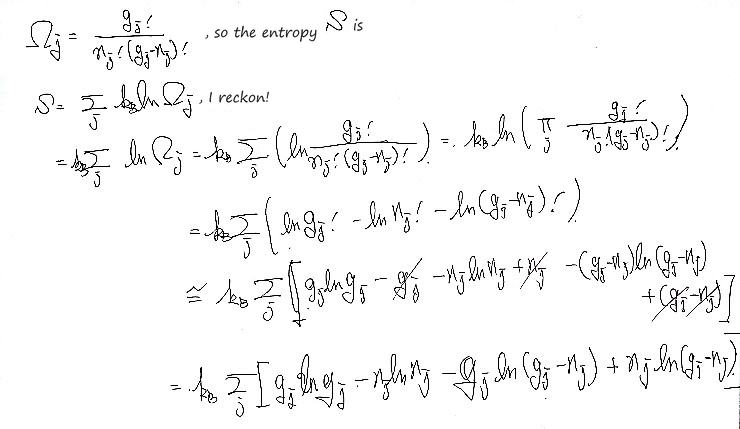
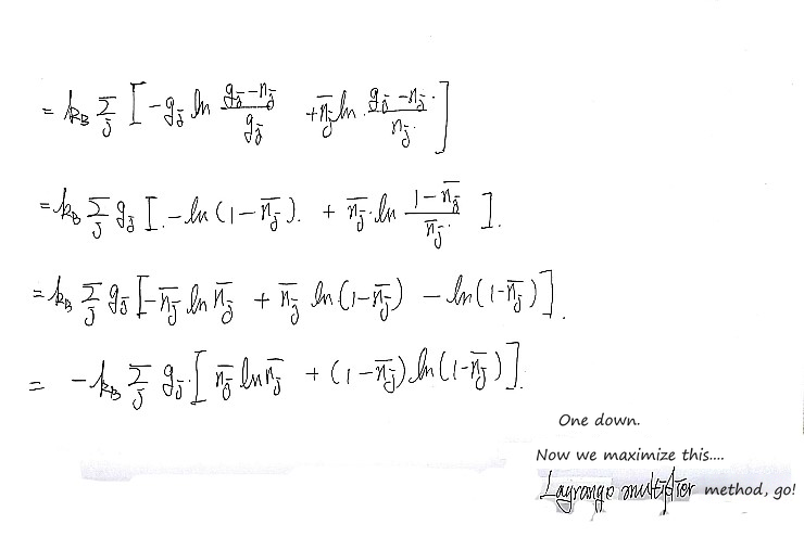
Multiplying the counts for the different energy groups gives the total count; taking its logarithm turns that product into the entropy sum. The sheets then use Stirling’s approximation for large counts. With $f_j=n_j/g_j$ (the $\bar n_j$ on the sheets), the result is

$$ \frac{S}{k_B}=-\sum_jg_j\big[f_j\ln f_j+(1-f_j)\ln(1-f_j)\big]. $$

So far this counts possible arrangements. To find the equilibrium occupation, we still have to maximize it without changing the total particle number or energy.

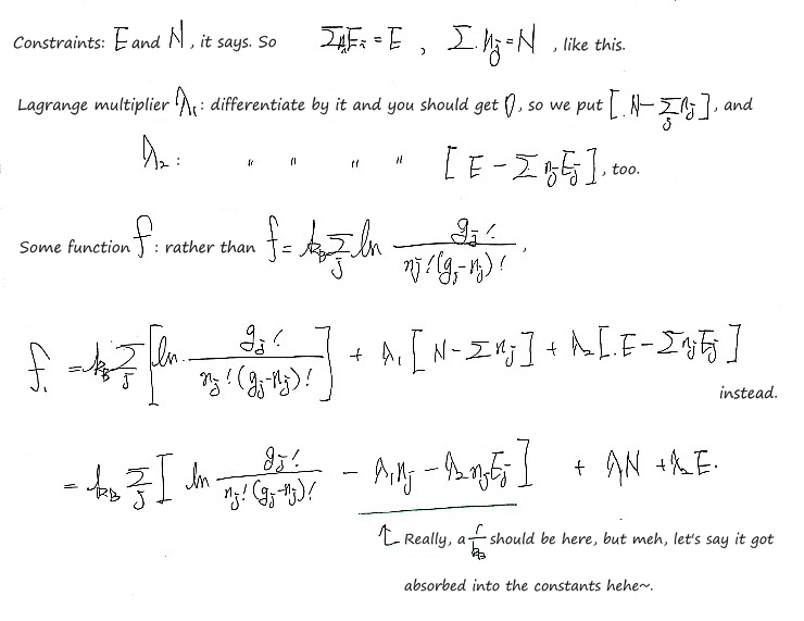
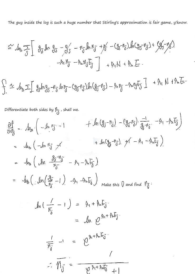
Those two restrictions are $\sum_jn_j=N$ and $\sum_jn_jE_j=E$. Maximizing $S/k_B-\alpha\sum_jn_j-\beta\sum_jn_jE_j$ gives

$$ \ln\frac{g_j-n_j}{n_j}=\alpha+\beta E_j, \qquad f_j=\frac{1}{e^{\alpha+\beta E_j}+1}. $$

The constants are fixed by the restrictions; in thermodynamic notation $\alpha=-\beta\mu$ and $\beta=1/(k_BT)$. This is the Fermi-Dirac function from the first problem again! The sheets absorb a factor of $k_B$ into their multiplier symbols; using $S/k_B$ here makes that convention explicit.

(b) Bosons

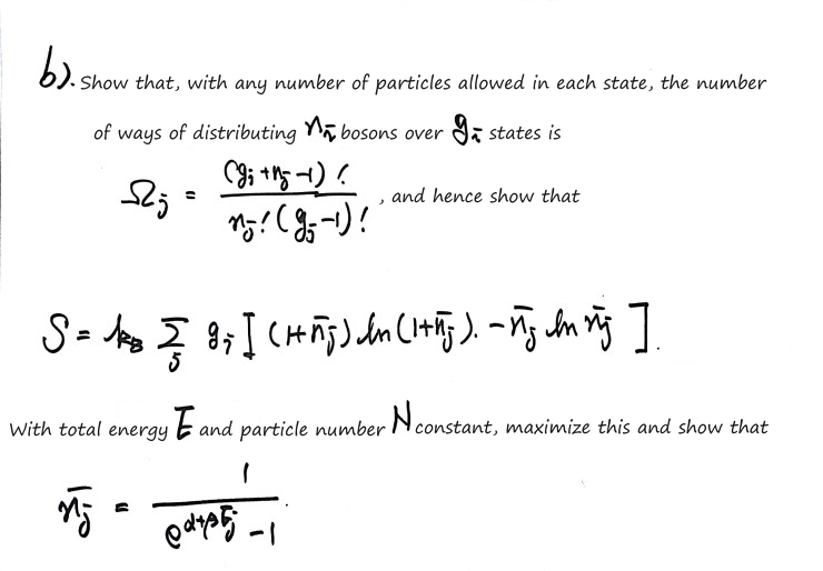
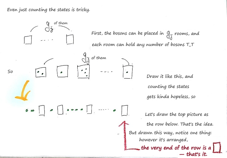
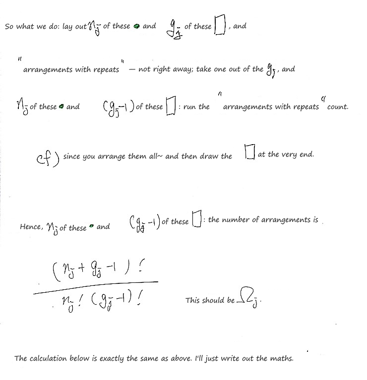
Now the occupancy restriction is gone: several bosons can share a state. Put $n_j$ identical dots in a row and use $g_j-1$ dividers to separate the $g_j$ states. Empty gaps are allowed. Choosing the positions of the dots among the dots and dividers gives

$$ \Omega_j=\binom{n_j+g_j-1}{n_j}. $$

That’s the little counting trick in the drawings. We haven’t changed what $g_j$ means; we’ve changed what is allowed inside each state.

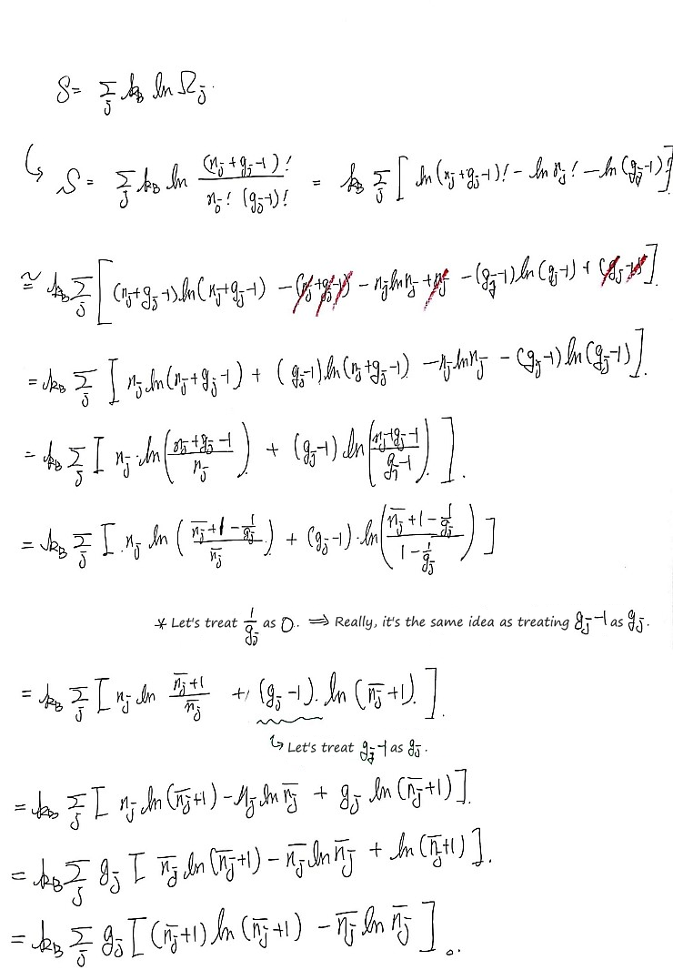
Taking $k_B\ln\Omega$ and using Stirling again gives, for large groups where the $-1$ terms can be neglected,

$$ \frac{S}{k_B}=\sum_jg_j\big[(1+f_j)\ln(1+f_j)-f_j\ln f_j\big]. $$

The factorial count above is exact. This smooth entropy expression is the large-number approximation used in the differentiation below.

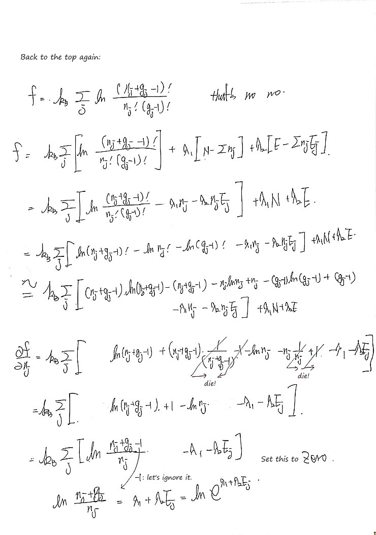
Keeping the same two restrictions, the derivative now gives

$$ \ln\frac{g_j+n_j}{n_j}=\alpha+\beta E_j, \qquad f_j=\frac{1}{e^{\beta(E_j-\mu)}-1}. $$

Compare the denominators: $+1$ for fermions, $-1$ for bosons. That small change came from the counting rules, not from a different temperature definition. Far out in the dilute tail, where $e^{\beta(E_j-\mu)}\gg1$, both reduce to $e^{-\beta(E_j-\mu)}$.

---

Heads-up. The figures here are the original notes, slips and all. A few things to watch for:

• In the statement of Prob 29.3, the Fermi-Dirac function is $f(E) = \frac{1}{2}\left(1 - \tanh\left(\frac{1}{2}\beta(E - \mu)\right)\right)$, without a second $\frac{1}{2}$ in front of the tanh; the next sheet writes it right.
• In the limits of Prob 29.3, the exponent keeps both $E$ and $\mu$: for $E-\mu\gg k_BT$, $f(E) \approx e^{-\beta(E - \mu)}$ (the Boltzmann tail), and for $\mu-E\gg k_BT$, $f(E) \approx 1 - e^{\beta(E - \mu)} \approx 1$. Dropping $E$ or $\mu$ from the exponent changes the result by a factor $e^{\beta\mu}$.
• The symmetry is point symmetry about $(\mu,1/2)$: $f(\mu+\delta)+f(\mu-\delta)=1$. The near-μ expansion assumes $|E-\mu|\ll k_BT$; the far limits must likewise be judged relative to $k_BT$, not just by comparing E and μ.